The probability integral transform
Problem
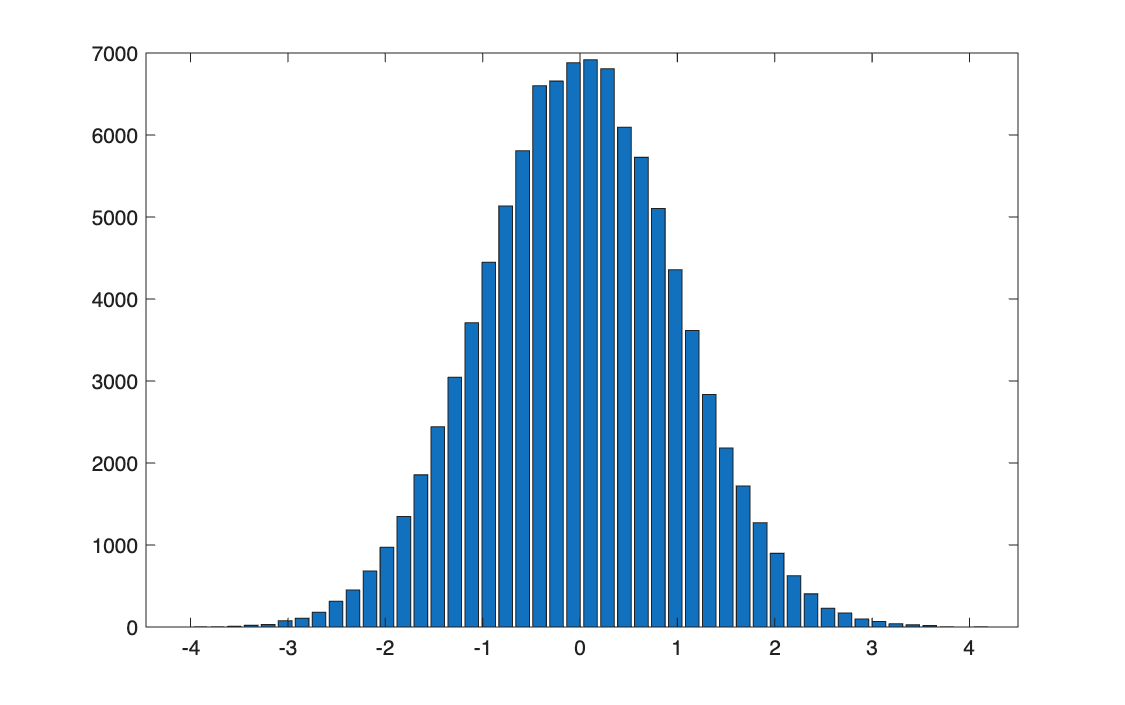
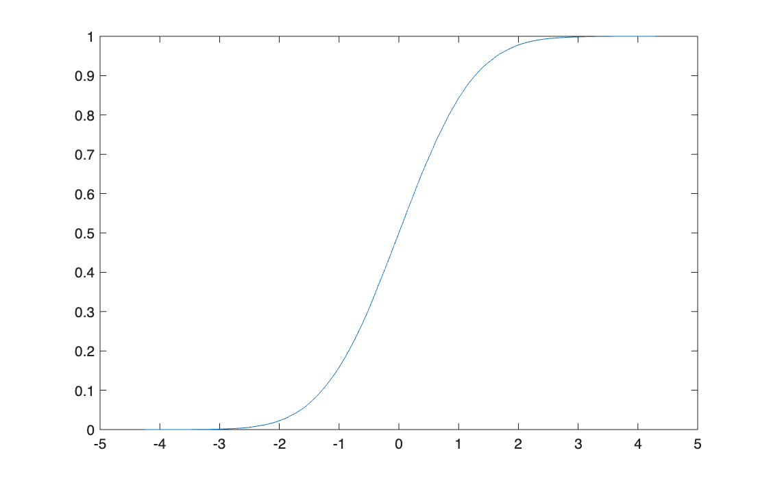
A function \(\varphi\) is given as a black box. Feed it 100,000 standard normal draws, study the distribution of the output (histogram, CDF, moments) and work out what \(\varphi\) does.
Method
The black box computes \(\varphi(z) = \tfrac12\big(1 + \operatorname{erf}(z/\sqrt2)\big)\), which is the standard normal CDF \(\Phi(z)\). For any continuous random variable \(Z\) with CDF \(F\),
\[
U = F(Z) \sim U[0, 1]
\]
because \(P(U \le u) = P(Z \le F^{-1}(u)) = F(F^{-1}(u)) = u\). This is the probability integral transform, and read backwards (\(Z = F^{-1}(U)\)) it is how uniform random numbers are turned into draws from any distribution.
Code
clear all, clc

%% 1

n = 100000;
nbins = 50;

Z = randn(n, 1);
p = ones(n, 1) / n;

%% 2

figure(1)
F_Empirical_pdf(Z, nbins);
print('-djpeg','G_MCmethodIn_pdf')

figure(2)
F_Empirical_cdf(Z, p);
print('-djpeg','G_MCmethodIn_cdf')

%% 3

Y = F_MCmethod(Z);

%% 4

[E_Y, Var_Y, Skew_Y, Kurt_Y] = F_SynteticIndices(Y)

figure(3)
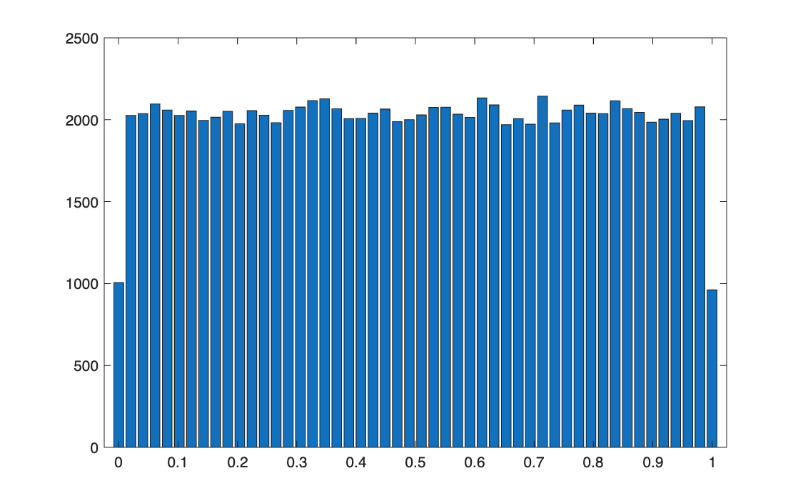
F_Empirical_pdf(Y, nbins);
print('-dtiff','G_MCmethodOut_pdf')

figure(4)
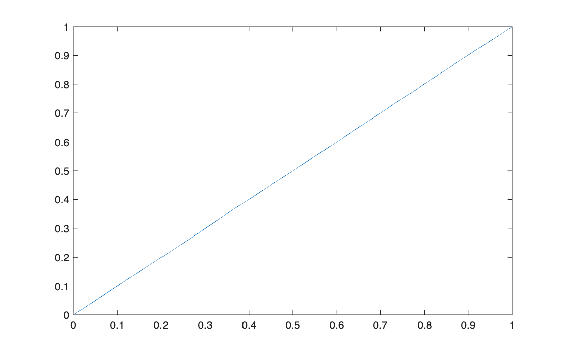
F_Empirical_cdf(Y, p);
print('-dtiff','G_MCmethodOut_cdf')

%% 5

% The output Y is distributed as a Uniform(0,1), not as the normal Z it
% started from. The charts show it: the empirical pdf is flat on [0,1] and
% the cdf grows linearly from (0,0) to (1,1). The summary statistics agree,
% matching those of a uniform (Section 2.6): mean ~ 0.5, variance ~ 0.083,
% skewness ~ 0 and kurtosis ~ 1.8. The reason is that the function phi used
% as a black box is the CDF of the standard normal: applied to samples of Z,
% which are exactly normal, it turns them into a Uniform(0,1).
import numpy as np
import matplotlib.pyplot as plt
from F_Empirical_pdf import F_Empirical_pdf
from F_Empirical_cdf import F_Empirical_cdf
from F_SynteticIndices import F_SynteticIndices
from F_MCmethod import F_MCmethod

# %% 1
n = 100000
nbins = 50

Z = np.random.randn(n)
p = np.ones(n) / n

# %% 2
plt.figure(1)
F_Empirical_pdf(Z, nbins)
plt.savefig('G_MCmethodIn_pdf.jpg')     # MATLAB: print('-djpeg', 'G_MCmethodIn_pdf')

plt.figure(2)
F_Empirical_cdf(Z, p)
plt.savefig('G_MCmethodIn_cdf.jpg')

# %% 3
Y = F_MCmethod(Z)

# %% 4
E_Y, Var_Y, Skew_Y, Kurt_Y = F_SynteticIndices(Y)

plt.figure(3)
F_Empirical_pdf(Y, nbins)
plt.savefig('G_MCmethodOut_pdf.tiff')

plt.figure(4)
F_Empirical_cdf(Y, p)
plt.savefig('G_MCmethodOut_cdf.tiff')

plt.show()

# %% 5
# Y is distributed as a Uniform(0,1), not as the normal Z it started from:
# flat pdf on [0,1], linear cdf, mean ~ 0.5, variance ~ 0.083, skewness ~ 0,
# kurtosis ~ 1.8. The black box phi is the standard normal CDF, and applied
# to normal samples it gives a Uniform(0,1).
import numpy as np
import matplotlib.pyplot as plt


def F_Empirical_cdf(x, p):
    index_sort = np.argsort(x)                  # MATLAB: [x_sort, index_sort] = sort(x)
    x_sort = x[index_sort]
    p_sort = p[index_sort]
    Emp_cdf = np.cumsum(p_sort)
    plt.step(x_sort, Emp_cdf, where='post')     # MATLAB: stairs(x_sort, Emp_cdf)
    return Emp_cdf
import numpy as np


def F_SynteticIndices(x):
    E_x = np.mean(x)
    print("E_x =", E_x)
    Var_x = np.mean((x - np.mean(x))**2)
    print("Var_x =", Var_x)
    Dev_x = np.sqrt(Var_x)
    Sk_x = np.mean(((x - np.mean(x)) / Dev_x)**3)
    print("Sk_x =", Sk_x)
    Ku_x = np.mean(((x - np.mean(x)) / Dev_x)**4)
    print("Ku_x =", Ku_x)
    return E_x, Var_x, Sk_x, Ku_x
In MATLAB, the helper functions F_Empirical_pdf, F_Empirical_cdf and F_SynteticIndices are
the ones shown in Part II.
Results
| Output \(Y\) | Sample | Uniform on [0, 1] |
|---|---|---|
| Mean | 0.4998 | 0.5 |
| Variance | 0.0831 | 0.0833 |
| Skewness | −0.0012 | 0 |
| Kurtosis | 1.8014 | 1.8 |
Takeaways
- Applying a distribution's own CDF to its samples always gives a uniform: the output no longer carries any trace of the normal shape.
- The moments identify the result without looking at the code: a kurtosis of 1.8 and a variance of 1/12 are the signature of a uniform.
- The inverse direction is the practical one: it is how a Monte Carlo simulation produces draws from a distribution starting from uniform random numbers.