Internal rate of return¶

Course exercise 57 · Part I

Problem¶

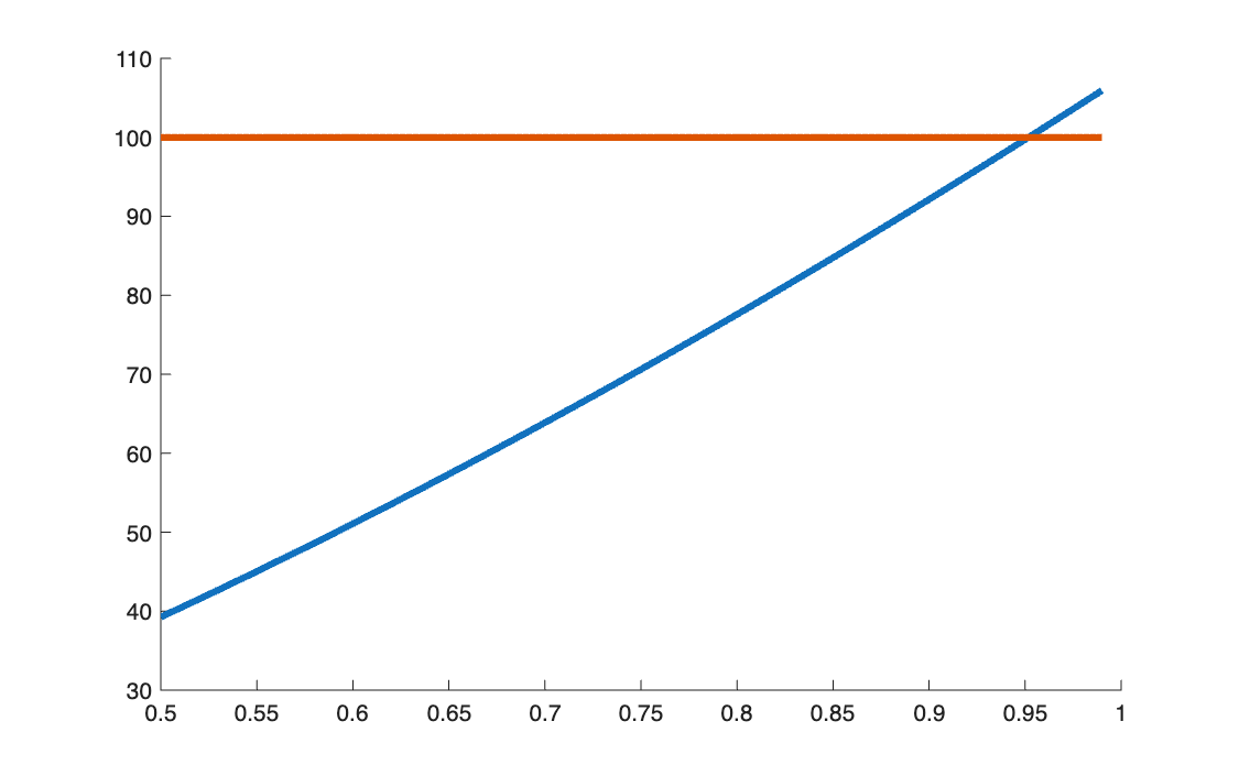
An investment costs 100 and pays 2.5 after 6 and 12 months and 102.5 after 18 months. Find its internal rate of return numerically, and show graphically where the solution lies.

Method¶

The IRR is the rate that sets the present value of all flows, cost included, to zero. Working with the discount factor \(v = 1/(1 + i)\), it is the root of:

\[ g(v) = \sum_k x_k\, v^{t_k} = 0, \qquad IRR = \frac{1}{v^*} - 1 \]

The root is found with fzero. For the chart, the same condition is split in two: the value of the future flows, \(f(v) = \sum_{k \ge 1} x_k v^{t_k}\), must equal the cost, 100. The IRR sits where the two curves cross.

Code¶

MATLABPython

S_exercise_57.m

clear all, clc

%% 1

x = [-100 2.5 2.5 102.5]

t = [ 0/12 6/12 12/12 18/12]

g = @(v) sum(x .* v.^(t))

v = fzero(g, 0.5)

IRR = (1 / v -1 ) * 100

% preparation for the plot

f = @(v) sum(x(2:end) .* v.^(t(2:end))) % the text says to start from k = 1, so the first flow is dropped

n = 1000

t = linspace(0.5, 0.99, n)

for k = 1 : n

    f_v(k) = f(t(k))

end

y = -x(1)

y_line = y * ones(1, n)

% plotting

figure(1)
hold on
plot(t, f_v, linewidth=3)
plot(t, y_line, linewidth=3)
hold off

% The intersection of f(v) and y is the discount factor v*
% that sets g(v) to zero, from which the IRR is obtained

S_exercise_57.py

import numpy as np
import matplotlib.pyplot as plt
from scipy.optimize import fsolve       # MATLAB's fzero: finds where a function is zero

# %% 1

x = np.array([-100, 2.5, 2.5, 102.5])
t = np.array([0/12, 6/12, 12/12, 18/12])

g = lambda v: np.sum(x * v**t)          # MATLAB: g = @(v) sum(x .* v.^(t))   (lambda = anonymous function)

v = fsolve(g, 0.5)[0]                   # MATLAB: fzero(g, 0.5)   ([0] takes the number out of the result)
print("v =", v)

IRR = (1 / v - 1) * 100
print("IRR =", IRR)

# preparation for the plot

f = lambda v: np.sum(x[1:] * v**t[1:])  # the text says to start from k = 1, so the first flow is dropped
                                        # MATLAB: x(2:end)  ->  Python: x[1:]

n = 1000
v_grid = np.linspace(0.5, 0.99, n)      # grid of discount factors
# (the MATLAB version reuses t for this grid. Not here: a Python lambda reads t when it
#  is called, not when it is created, so f would see the new t and break)

f_v = np.zeros(n)
for k in range(n):
    f_v[k] = f(v_grid[k])

y = -x[0]                               # MATLAB: -x(1)
y_line = y * np.ones(n)

# plotting
plt.figure(1)
plt.plot(v_grid, f_v, linewidth=3)
plt.plot(v_grid, y_line, linewidth=3)
plt.show()

# The intersection of f(v) and y is the discount factor v*
# that sets g(v) to zero, from which the IRR is obtained

Results¶

\(v^* = 0.9518\), so IRR = 5.0625% a year.

Value of the future flows against the discount factor, crossing the cost of 100

Takeaways¶

The result can be checked by hand: 2.5 every six months on 100 is 2.5% per half-year, and \(1.025^2 - 1 = 5.0625\%\).
Solving in \(v\) instead of \(i\) turns the problem into finding the root of a polynomial-like function, which fzero handles from any reasonable starting point.