Written exam, 16 July 2026¶

Computational Finance · exam session of 16 July 2026

Three tasks, solved in MATLAB under exam conditions: the value of an annuity, a European call priced with Black–Scholes and with Monte Carlo, and a MinMax efficient frontier.

The code below is exactly as submitted. The only changes are the removal of the header line with my student details, the translation of the comments into English, and the removal of the blank line that followed every line of code in the saved files. It was not reviewed before publication; the problems found on review are listed at the end of the page, with the correct numbers, instead of being fixed in the code.

Task 1 · Present value of an annuity¶

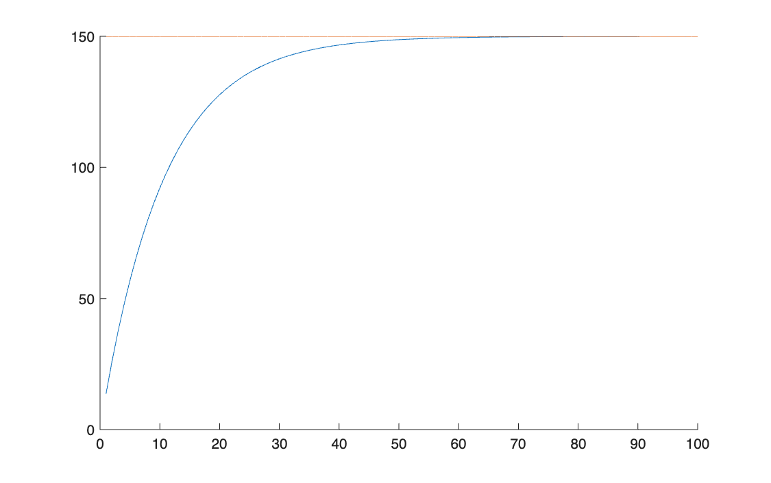
An annuity pays 15 a year for 20 years at 10%. Compute its value with the closed form, with a function and with a loop, then plot the value against the number of payments.

S_Annuity.mF_Annuity.m

clear all, clc

i = 0.10
R = 15
n = 20
v = 1 / (1 + i)
V_0 = R * v * ((1 - v^n) / (1 - v))
%
V_0_funct = F_Annuity(i,R,n)
%
V_0_for = R*v(1);
for k = 2 : n
    V_0_for = V_0_for +  R * v^k;
end
V_0_for
%
n_graph = 1:100;
asympt = R / i
T = R * v * (1 - v.^n_graph) / (1 - v)
figure(1)
hold on
plot(n_graph, T)
plot(n_graph, asympt*ones(1, 100))
 print('G_Annuity.jpg', '-djpeg')

function [V_0] = F_Annuity(i,R,n)
v = 1 / (1 + i)
V_0 = R * v * ((1 - v^n) / (1 - v))
end

The three methods agree: 127.7035. The perpetuity value, the asymptote, is \(R/i = 150\).

Annuity value against the number of payments

Task 2 · European call: Black–Scholes against Monte Carlo¶

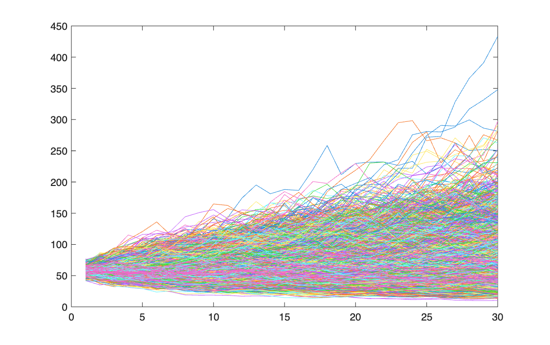
Price a two-year call with \(S_0 = 57\), \(K = 62\), \(r = 9\%\), \(\sigma = 32\%\), with the closed form and by simulating 10,000 paths of 30 steps.

S_MCvsBS.mF_formulaBS.mF_Montecarlo_def.m

clear all, clc

K = 62
S_0 = 57
r = 0.09
T = 2
sigma = 0.32
n = 10000
m = 30
%
Call_price_BS = F_formulaBS(S_0, K, r, sigma, T)
Call_price_M = F_Montecarlo_def(S_0, sigma, r, T, K, n, m)
%
% the GBM is plotted inside F_Montecarlo_def

function [Call_price_BS] = F_formulaBS(S_0, K, r, sigma, T)
d1 = (log(S_0 ./ K) + (r + sigma.^2 /2) .* T) ./ (sigma .* sqrt(T))
d2 = d1 - sigma .* sqrt(T)
%
nd1 = 1/2 * (1 + erf(d1 / sqrt(2)))
nd2 = 1/2 * ( 1 + erf(d2 / sqrt(2)))
%
Call_price_BS = S_0 .* nd1 - K .* exp(-r * T) .* nd2
end

function [Call_price_M] = F_Montecarlo_def(S_0, sigma, r, T, K, n, m)
Dt = T / m
Z = randn(n, m)
dx = (r - (sigma^2 / 2)) * Dt + sigma * sqrt(Dt) * Z
S_T = S_0 * exp(cumsum(dx, 2))
Call_price_M = exp(-r * T) * mean(max(S_T - K, 0));
%Put_price = exp(-r * T) * mean(max(K - S_T, 0));
Call_price_M
plot(S_T')
print('G_MotoBrownGeom.jpg', '-djpeg')
end

The closed form gives 12.5577, which is correct. The Monte Carlo function returns 30 numbers, rising from 0.38 to 12.47, instead of one price; see below.

The 10,000 simulated price paths

Task 3 · MinMax efficient frontier¶

On 10 NASDAQ-100 stocks and 289 returns, build the frontier that minimises the worst loss for each target return, and plot the number of stocks selected.

S_MinMax.m

clear all, clc

%
L = readtable("NASDAQ100.xlsx");
times = L{:, 1}
P = L{:, 2:end};
P_cut = P(end-289:end, 1:10);
RR = diff(P_cut) ./ P_cut(1:end-1, :); % R_cut
mu = mean(RR);
%
[T, n] = size(RR)
%
f = [zeros(n, 1); -1];
A = [-RR, ones(T, 1)];
b = zeros(T, 1);
Aeq = [ones(1, n), 0];
beq = 1;
LB = [zeros(n, 1); -inf];
[x_min, var_min] = linprog(f,A,b,Aeq,beq,LB,[]);
x_min = x_min(1:n);
eta_min = mu * x_min
eta_max = max(mu)
eta = linspace(eta_min, eta_max, 50);
%
options = optimset(MaxIter=1.e7, TolFun=1.e-10, TolX = 1.e-10)
Aeq_ = [mu, 0; ones(1, n), 0];
for k = 1 : length(eta)
    beq_ = [eta(k); 1];
    [x_port(:, k), var_port(:, k)] = linprog(f,A,b,Aeq_,beq_,LB,[], [], options); %Risk_minMax
end
%
xlswrite('FrontieraMinMax.xls','eta', 'var_port')
%
figure(1)
plot(var_port, eta, linewidth = 2)
xlabel('Risk_MinMax')
ylabel('eta')
title('Modello MinMax')
print('G_FrontieraMinMax.jpg', '-djpeg')
%
title_sort = sum(x_port > 1.e-5) % the number of stocks falls as the portfolio risk grows
figure(2)
plot(title_sort, eta)
print('G_NumAssSelected.jpg', '-djpeg')

With current MATLAB the script stops at the frontier loop; see below. With that one call fixed, the model is right: the worst loss goes from 7.85% for the minimum-risk portfolio (2 stocks, mean return 0.108% per period) to 18.45% for the best single stock (0.374%), and the number of stocks falls from 2 to 1 as the target return rises, as the comment in the code says.

Problems found on review¶

Task	Where	What is wrong	Effect	Correct result
2	`F_Montecarlo_def`	the payoff is averaged over the whole \(n \times m\) matrix of paths instead of the final prices `S_T(:, end)`	30 "prices", one per time step, all discounted as if they matured at \(T\)	the last one, 12.4676, is the Monte Carlo price, within simulation error of 12.5577
3	frontier loop	`linprog(f, A, b, Aeq_, beq_, LB, [], [], options)` passes a starting point (the second `[]`) before the options; current MATLAB releases reject it ("does not accept X0")	the script stops; no frontier is plotted	worst loss from 7.85% to 18.45%, as above
3	`xlswrite`	`xlswrite('FrontieraMinMax.xls', 'eta', 'var_port')` writes the text `'eta'` into a sheet named `var_port`	the results are not saved	`xlswrite(file, [eta; var_port])`

Task 1 and the Black–Scholes function of task 2 are correct as submitted.