Mean-CVaR efficient frontier¶

Course exercise 139 · Part II

Problem¶

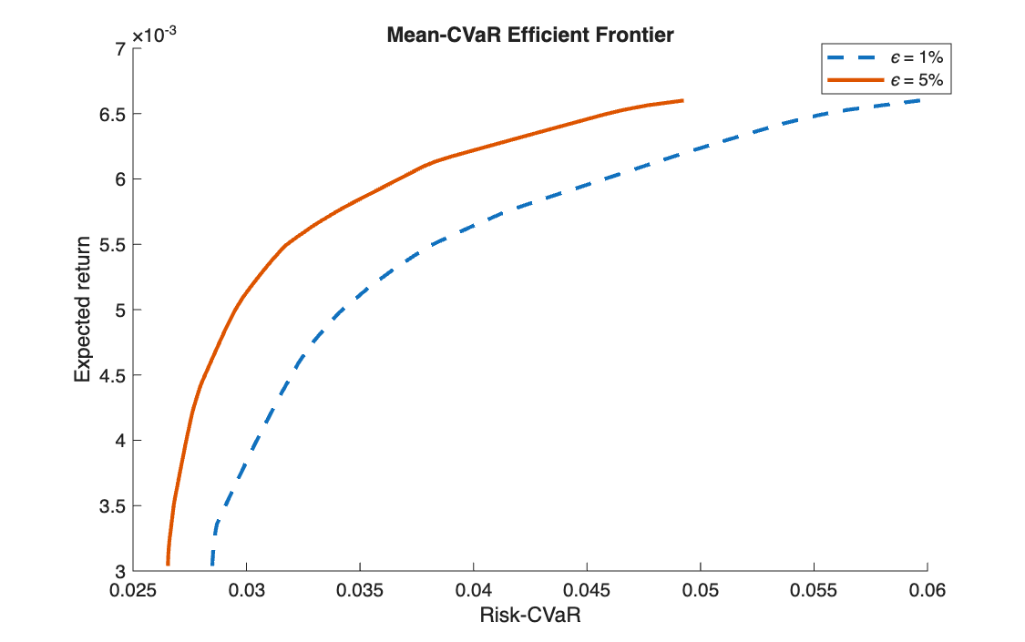
On the same EURO STOXX 50 data, measure risk with the Conditional Value at Risk at 1% and at 5%, and build the two efficient frontiers.

Method¶

CVaR can be minimised as a linear program (Rockafellar–Uryasev). With a threshold variable \(\alpha\) and one excess variable \(y_t \ge 0\) per scenario:

\[ \min_{x,\,y,\,\alpha}\ \alpha + \frac{1}{\varepsilon T}\sum_{t=1}^{T} y_t \quad \text{s.t.} \quad y_t \ge -r_t^\top x - \alpha,\quad \mu^\top x = \eta,\quad \mathbf{1}^\top x = 1,\quad x \ge 0 \]

At the optimum \(\alpha\) is the VaR and the objective is the CVaR. The same grid of target returns is used for both levels of \(\varepsilon\), so the two frontiers can be compared point by point.

Code¶

MATLABPython

S_exercise_139.m

clear, clc

%% 1

A      = readtable('weekly_EUROSTOXX50_price_time.txt');
dates  = A{:, 1};
P      = A{:, 2:end};
RR     = diff(P) ./ P(1:end-1, :);
[T, n] = size(RR);                  % T = weeks, n = stocks

%% 2

mu = mean(RR);

%% 3

A = [-RR, -eye(T), -ones(T,1)];
b  = zeros(T, 1);
lb = [zeros(n+T, 1); -inf];

f1 = [zeros(n, 1); ones(T, 1)/(0.01*T); 1];
f5 = [zeros(n, 1); ones(T, 1)/(0.05*T); 1];

% The eta grid is SINGLE and shared: one solve fixes its lower end (using f5)
Aeq     = [ones(1,n), zeros(1,T), 0];   beq = 1;
x_min   = linprog(f5, A, b, Aeq, beq, lb, []);
eta_min = mu * x_min(1:n);
eta_max = max(mu);

%% 4

N   = 100;
eta = linspace(eta_min, eta_max, N);

%% 5

Aeq_ = [mu,        zeros(1,T), 0;
        ones(1,n), zeros(1,T), 0];

Risk_CVaR_1 = NaN(1, N);
Risk_CVaR_5 = NaN(1, N);

for k = 1:N
    beq_ = [eta(k); 1];
    [~, Risk_CVaR_1(k)] = linprog(f1, A, b, Aeq_, beq_, lb, []);   % CVaR 1%
    [~, Risk_CVaR_5(k)] = linprog(f5, A, b, Aeq_, beq_, lb, []);   % CVaR 5%
end

%% 6

figure(1);
hold on
plot(Risk_CVaR_1, eta, '--', LineWidth=2)
plot(Risk_CVaR_5, eta, '-',  LineWidth=2)
xlabel('Risk-CVaR'); ylabel('Expected return')
title('Mean-CVaR Efficient Frontier')
legend('\epsilon = 1%', '\epsilon = 5%')
print('CVaREF.jpg', '-djpeg')

S_exercise_139.py

import numpy as np
import matplotlib.pyplot as plt
from scipy.optimize import linprog

# %% 1
A = np.loadtxt('weekly_EUROSTOXX50_price_time.txt')
dates = A[:, 0]
P = A[:, 1:]
RR = np.diff(P, axis=0) / P[:-1, :]
T, n = RR.shape                         # T = weeks, n = stocks

# %% 2
mu = np.mean(RR, axis=0)

# %% 3
A = np.hstack([-RR, -np.eye(T), -np.ones((T, 1))])   # MATLAB: [-RR, -eye(T), -ones(T,1)]
b = np.zeros(T)
lb = [(0, None)] * (n + T) + [(None, None)]           # weights and excesses >= 0; threshold free

f1 = np.concatenate([np.zeros(n), np.ones(T) / (0.01 * T), [1]])
f5 = np.concatenate([np.zeros(n), np.ones(T) / (0.05 * T), [1]])

# The eta grid is single and shared: one solve fixes its lower end (using f5)
Aeq = np.concatenate([np.ones(n), np.zeros(T), [0]]).reshape(1, -1)
beq = [1]
x_min = linprog(f5, A_ub=A, b_ub=b, A_eq=Aeq, b_eq=beq, bounds=lb).x
eta_min = mu @ x_min[:n]
eta_max = np.max(mu)

# %% 4
N = 100
eta = np.linspace(eta_min, eta_max, N)

# %% 5
Aeq_ = np.vstack([np.concatenate([mu, np.zeros(T), [0]]),
                  np.concatenate([np.ones(n), np.zeros(T), [0]])])

Risk_CVaR_1 = np.zeros(N)
Risk_CVaR_5 = np.zeros(N)

for k in range(N):
    beq_ = [eta[k], 1]
    Risk_CVaR_1[k] = linprog(f1, A_ub=A, b_ub=b, A_eq=Aeq_, b_eq=beq_, bounds=lb).fun   # CVaR 1%
    Risk_CVaR_5[k] = linprog(f5, A_ub=A, b_ub=b, A_eq=Aeq_, b_eq=beq_, bounds=lb).fun   # CVaR 5%

print("CVaR 1%:", Risk_CVaR_1[0], "..", Risk_CVaR_1[-1], "  CVaR 5%:", Risk_CVaR_5[0], "..", Risk_CVaR_5[-1])

# %% 6
plt.figure(1)
plt.plot(Risk_CVaR_1, eta, '--', linewidth=2)
plt.plot(Risk_CVaR_5, eta, '-', linewidth=2)
plt.xlabel('Risk-CVaR'); plt.ylabel('Expected return')
plt.title('Mean-CVaR Efficient Frontier')
plt.legend(['epsilon = 1%', 'epsilon = 5%'])
plt.savefig('CVaREF.jpg')
plt.show()

Results¶

	Lowest CVaR	Highest CVaR
\(\varepsilon = 5\%\)	2.65%	4.93%
\(\varepsilon = 1\%\)	2.85%	5.97%

Weekly figures, over target returns from 0.304% to 0.660%.

Mean-CVaR efficient frontiers at 1% and 5%

Takeaways¶

CVaR is the risk measure of this part that is both coherent (it rewards diversification) and linear-programmable.
The 1% frontier lies to the right of the 5% one: looking deeper into the tail sees larger losses for the same portfolio.
With 262 weekly scenarios, the 1% tail is only about 3 observations, so the 1% frontier is close to the MaxLoss one.

Comparing the risk measures¶

The four frontiers of this part use the same 47 stocks and the same 262 weeks:

Page	Risk measure	Problem type
Mean-variance	variance	quadratic
Mean-MAD	mean absolute deviation	linear
Mean-MaxLoss	worst weekly loss	linear
Mean-CVaR	average loss in the worst ε of weeks	linear