Mean-MaxLoss efficient frontier
Problem
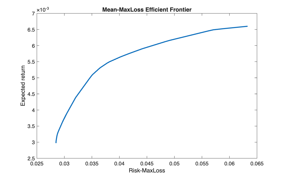
On the same EURO STOXX 50 data, measure risk as the worst weekly return observed in the sample, and build the frontier that minimises that worst loss for each target return.
Method
Maximising the worst portfolio return is linear with one auxiliary variable \(d\), a lower bound on the portfolio return in every scenario:
\[
\max_{x,\,d}\ d
\quad \text{s.t.} \quad
d \le r_t^\top x \ \ \forall t,\quad
\mu^\top x = \eta,\quad \mathbf{1}^\top x = 1,\quad x \ge 0
\]
At the optimum \(d\) is the worst return, and \(-d\) is the maximum loss. linprog minimises, so
the objective is \(-d\).
Code
clear all, clc

%% 1

A = readtable('weekly_EUROSTOXX50_price_time.txt');
times = A{:, 1};
P = A{:, 2:end};

%% 2

RR = diff(P) ./ P(1:end-1, :);
[T, n] = size(RR);

%% 3

mu = mean(RR);

%% 4

f  = [zeros(1, n), -1];        % minimise -d  ->  maximise d (= -MaxLoss)
A_ = [-RR, ones(T, 1)];        % d - sum(r_t x) <= 0  for every t
b  = zeros(T, 1);
lb = [zeros(n, 1); -inf];      % x >= 0 (no short selling); d free
ub = [];

% minimum risk (budget only)
Aeq = [ones(1, n), 0];
beq = 1;

[X0, fo] = linprog(f, A_, b, Aeq, beq, lb, ub);
x_min   = X0(1:n);
eta_min = mu * x_min;
eta_max = max(mu);

%% 5

N   = 100;
eta = linspace(eta_min, eta_max, N);

%% 6

Risk_MaxLoss = NaN(1, N);

Aeq_ = [mu,         0;          % return constraint
        ones(1, n), 0];         % budget constraint

for k = 1:N
    beq_ = [eta(k); 1];
    [X_star, fo_star] = linprog(f, A_, b, Aeq_, beq_, lb, []);
    Risk_MaxLoss(k) = fo_star;
end

%% 7

figure(1)
plot(Risk_MaxLoss, eta, LineWidth=2)
xlabel('Risk-MaxLoss')
ylabel('Expected return')
title('Mean-MaxLoss Efficient Frontier')
import numpy as np
import matplotlib.pyplot as plt
from scipy.optimize import linprog

# %% 1
A = np.loadtxt('weekly_EUROSTOXX50_price_time.txt')
times = A[:, 0]
P = A[:, 1:]

# %% 2
RR = np.diff(P, axis=0) / P[:-1, :]
T, n = RR.shape

# %% 3
mu = np.mean(RR, axis=0)

# %% 4
f = np.concatenate([np.zeros(n), [-1]])          # minimise -d  ->  maximise d (= -MaxLoss)
A_ = np.hstack([-RR, np.ones((T, 1))])           # d - sum(r_t x) <= 0  for every t
b = np.zeros(T)
lb = [(0, None)] * n + [(None, None)]            # x >= 0 (no short selling); d free

# minimum risk (budget only)
Aeq = np.concatenate([np.ones(n), [0]]).reshape(1, -1)
beq = [1]

res = linprog(f, A_ub=A_, b_ub=b, A_eq=Aeq, b_eq=beq, bounds=lb)
X0 = res.x
fo = res.fun
x_min = X0[:n]
eta_min = mu @ x_min
eta_max = np.max(mu)

# %% 5
N = 100
eta = np.linspace(eta_min, eta_max, N)

# %% 6
Risk_MaxLoss = np.zeros(N)

Aeq_ = np.vstack([np.concatenate([mu, [0]]),           # return constraint
                  np.concatenate([np.ones(n), [0]])])  # budget constraint

for k in range(N):
    beq_ = [eta[k], 1]
    res = linprog(f, A_ub=A_, b_ub=b, A_eq=Aeq_, b_eq=beq_, bounds=lb)
    Risk_MaxLoss[k] = res.fun

print("fo =", fo, " eta_min =", eta_min, " MaxLoss at the top =", Risk_MaxLoss[-1])

# %% 7
plt.figure(1)
plt.plot(Risk_MaxLoss, eta, linewidth=2)
plt.xlabel('Risk-MaxLoss')
plt.ylabel('Expected return')
plt.title('Mean-MaxLoss Efficient Frontier')
plt.show()
Results
The minimum-MaxLoss portfolio loses at most 2.85% in its worst week, with an expected return of 0.297%, holding 10 stocks. At the top of the frontier the worst week costs 6.33%.
Takeaways
- The worst case of the sample becomes an explicit constraint: only one variable is added, and one constraint per week.
- It is the most conservative measure of the set: it looks at a single observation, the worst, and ignores how often bad weeks happen.
- That same feature makes it unstable: one extreme week in or out of the sample can move the whole frontier.