Are prices or returns stationary? Four Dow Jones stocks, 2006–2026
Problem
Take twenty years of daily prices for four Dow Jones stocks (Apple, JPMorgan, Chevron, Johnson & Johnson), compute their returns and descriptive statistics, and test empirically whether prices and returns are stationary, by splitting the history in two and comparing the distributions of the two halves.
Method
A process is stationary if its probability distribution does not change over time. An empirical check: split the sample into Period 1 (January 2006 – December 2015, 2,513 days) and Period 2 (January 2016 – April 2026, 2,576 days), then compare the histograms and the first four moments of each period, first for prices, then for linear returns.
Code
clear all; close all; clc;

% The exercise uses the file DowJones_price.xlsx. Since the stocks named in
% exercise 119 are not in it, four others are chosen: AAPL, JPM, CVX, JNJ.


% Point 1 — Import and returns

    T = readtable("DowJones_price.xlsx");

    % --- Prices ---
    % T{:, 'col'} extracts the column as a plain numeric vector, without labels.
    % Curly braces are what let us work with vectors and matrices.
    AAPL_prices = T{:, 'AAPL_OQ'};
    JPM_prices  = T{:, 'JPM_N'};
    CVX_prices  = T{:, 'CVX_N'};
    JNJ_prices  = T{:, 'JNJ_N'};

    % --- Linear returns ---
    % Technical note: in exercise 117 we had a row vector; here we have column
    % vectors. diff recognises the shape and works in both cases.
    AAPL_returns = diff(AAPL_prices) ./ AAPL_prices(1:end-1);
    JPM_returns  = diff(JPM_prices)  ./ JPM_prices(1:end-1);
    CVX_returns  = diff(CVX_prices)  ./ CVX_prices(1:end-1);
    JNJ_returns  = diff(JNJ_prices)  ./ JNJ_prices(1:end-1);

    % --- Full returns matrix, saved to file ---
    Returns = [AAPL_returns, JPM_returns, CVX_returns, JNJ_returns];
    writematrix(Returns, 'DowJones_returns.xlsx');


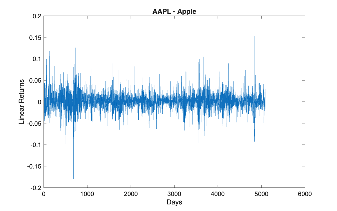
% Point 2 — Plot of the returns

    figure(1)
    plot(AAPL_returns);
    title('AAPL - Apple');      ylabel('Linear Returns'); xlabel('Days');

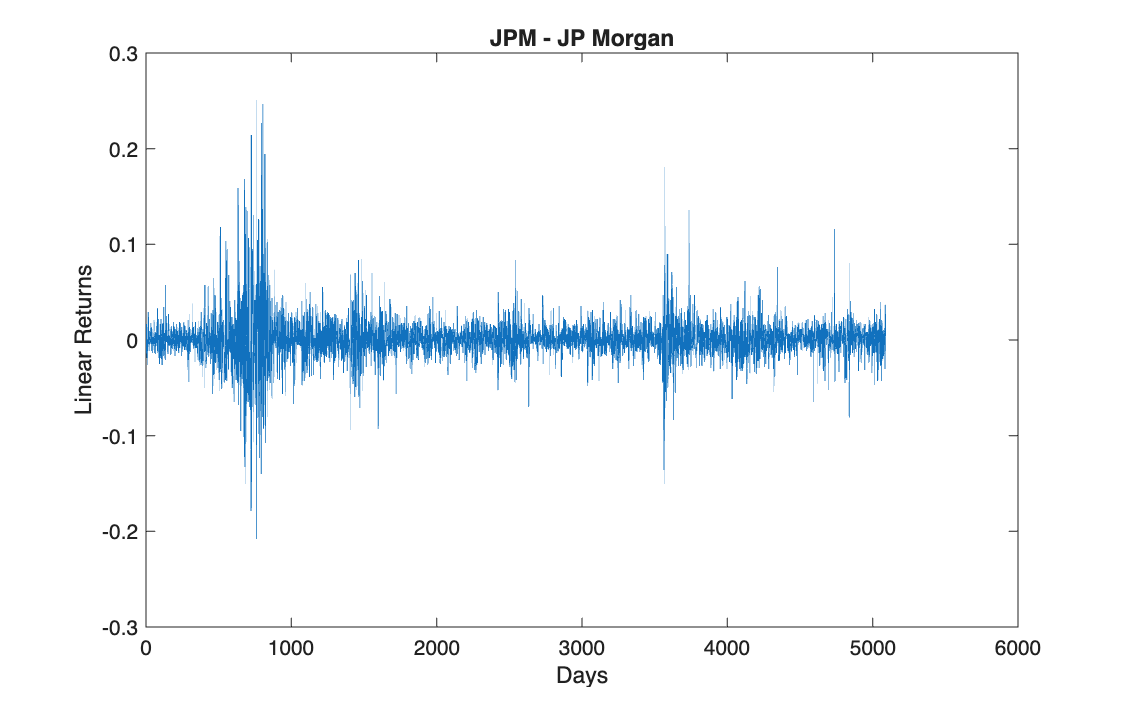
    figure(2)
    plot(JPM_returns);
    title('JPM - JP Morgan');   ylabel('Linear Returns'); xlabel('Days');

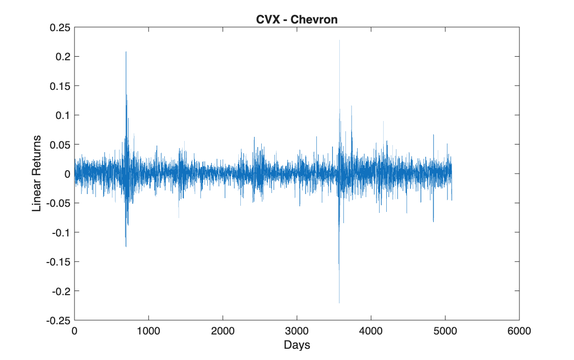
    figure(3)
    plot(CVX_returns);
    title('CVX - Chevron');     ylabel('Linear Returns'); xlabel('Days');

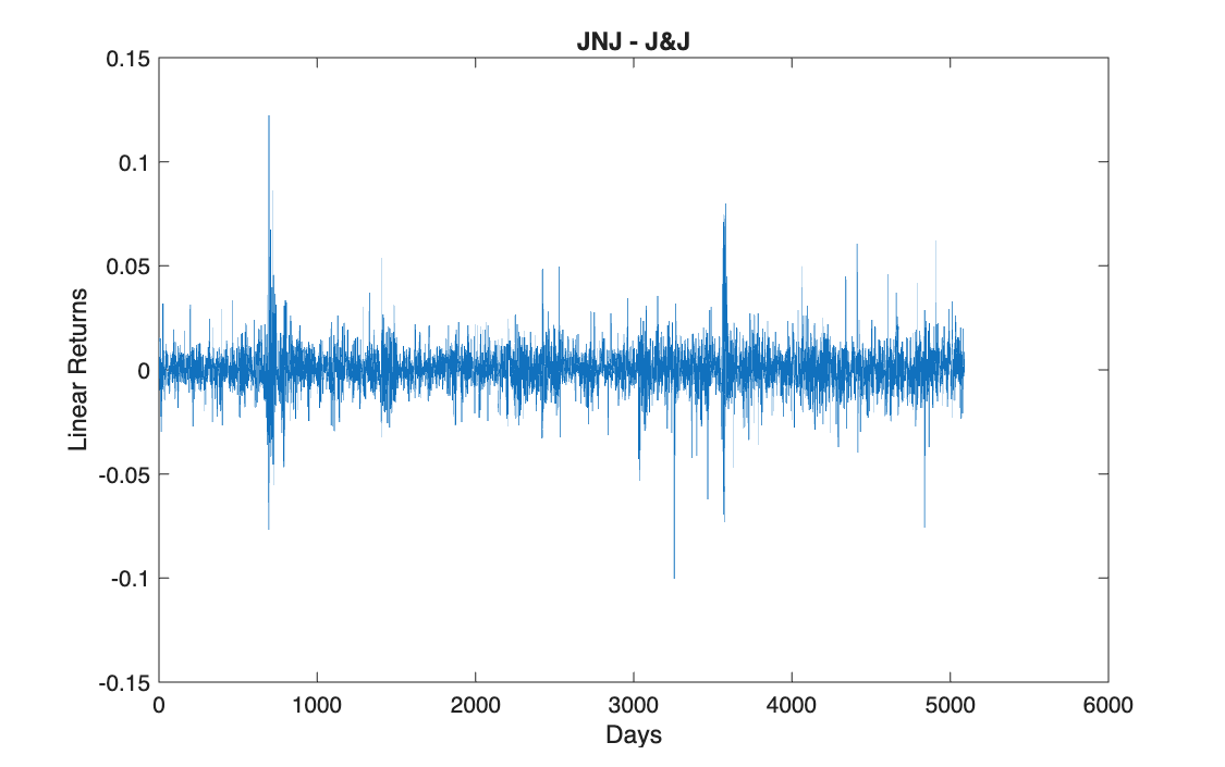
    figure(4)
    plot(JNJ_returns);
    title('JNJ - J&J');         ylabel('Linear Returns'); xlabel('Days');


% Point 3 — Descriptive statistics

    % mean(X, 1): works along dimension 1 (rows): collapses all the rows into
    % one value, column by column -> one statistic per asset.
    % With 2 it would work by row.
    Exp_returns = mean(Returns, 1);
    Std         = std(Returns,  1);
    Skew        = skewness(Returns, 1);
    Kurt        = kurtosis(Returns, 1);
    Sigma       = cov(Returns);

    % save 'DowJones_Workspace.mat'   % uncomment to save the workspace


% Point 4 — Stationarity analysis


    % Stationarity requires the probability distribution not to change over
    % time. To check it empirically, the history is split into two
    % sub-periods and their distributions and summary statistics are compared.
    % Split: Period 1 = 2006-2015 (2513 obs) | Period 2 = 2016-2026 (2576 obs)


    split   = 2513;
    split_r = split - 1;    % there is one return fewer than prices

    % --- Split prices ---
    AAPL_p1 = AAPL_prices(1:split);        AAPL_p2 = AAPL_prices(split+1:end);
    JPM_p1  = JPM_prices(1:split);         JPM_p2  = JPM_prices(split+1:end);
    CVX_p1  = CVX_prices(1:split);         CVX_p2  = CVX_prices(split+1:end);
    JNJ_p1  = JNJ_prices(1:split);         JNJ_p2  = JNJ_prices(split+1:end);

    % --- Split returns ---
    AAPL_r1 = AAPL_returns(1:split_r);     AAPL_r2 = AAPL_returns(split_r+1:end);
    JPM_r1  = JPM_returns(1:split_r);      JPM_r2  = JPM_returns(split_r+1:end);
    CVX_r1  = CVX_returns(1:split_r);      CVX_r2  = CVX_returns(split_r+1:end);
    JNJ_r1  = JNJ_returns(1:split_r);      JNJ_r2  = JNJ_returns(split_r+1:end);


% 4.1 PDF of the prices

    nbins_p = 50;

    figure(5)
    subplot(1,2,1); F_es99(AAPL_p1, nbins_p); title('AAPL - Prices PDF 2006-2015'); xlabel('Price'); ylabel('Frequency');
    subplot(1,2,2); F_es99(AAPL_p2, nbins_p); title('AAPL - Prices PDF 2016-2026'); xlabel('Price'); ylabel('Frequency');
    sgtitle('AAPL - Price Distribution', 'FontSize', 14, 'FontWeight', 'bold');

    figure(6)
    subplot(1,2,1); F_es99(JPM_p1, nbins_p); title('JPM - Prices PDF 2006-2015'); xlabel('Price'); ylabel('Frequency');
    subplot(1,2,2); F_es99(JPM_p2, nbins_p); title('JPM - Prices PDF 2016-2026'); xlabel('Price'); ylabel('Frequency');
    sgtitle('JPM - Price Distribution', 'FontSize', 14, 'FontWeight', 'bold');

    figure(7)
    subplot(1,2,1); F_es99(CVX_p1, nbins_p); title('CVX - Prices PDF 2006-2015'); xlabel('Price'); ylabel('Frequency');
    subplot(1,2,2); F_es99(CVX_p2, nbins_p); title('CVX - Prices PDF 2016-2026'); xlabel('Price'); ylabel('Frequency');
    sgtitle('CVX - Price Distribution', 'FontSize', 14, 'FontWeight', 'bold');

    figure(8)
    subplot(1,2,1); F_es99(JNJ_p1, nbins_p); title('JNJ - Prices PDF 2006-2015'); xlabel('Price'); ylabel('Frequency');
    subplot(1,2,2); F_es99(JNJ_p2, nbins_p); title('JNJ - Prices PDF 2016-2026'); xlabel('Price'); ylabel('Frequency');
    sgtitle('JNJ - Price Distribution', 'FontSize', 14, 'FontWeight', 'bold');

    % Results - PDF of the prices:
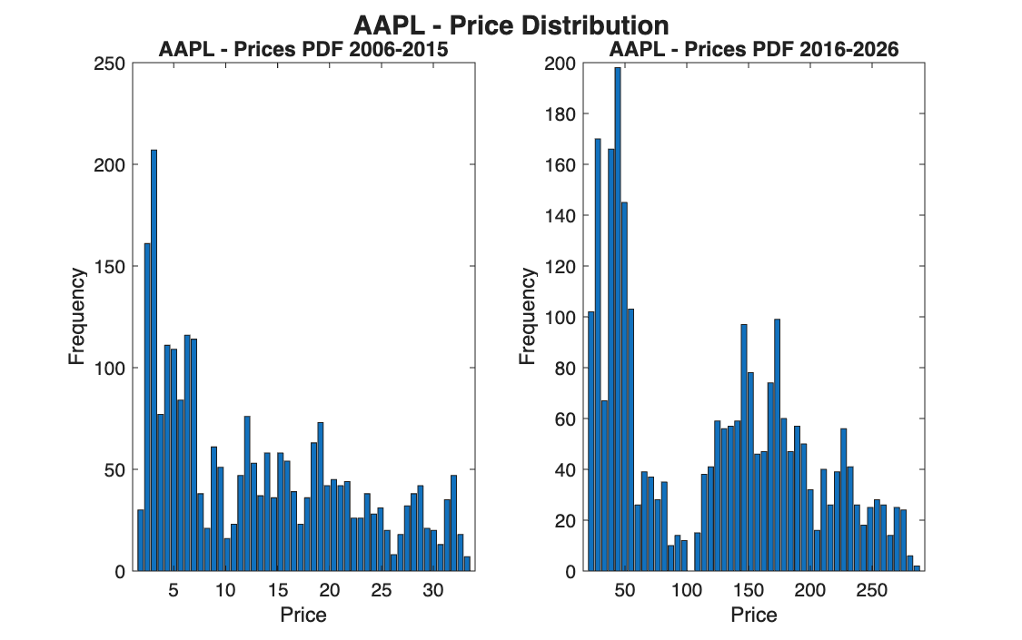
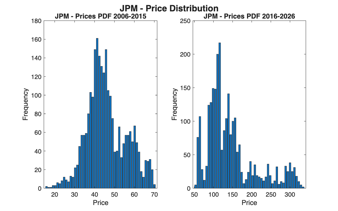
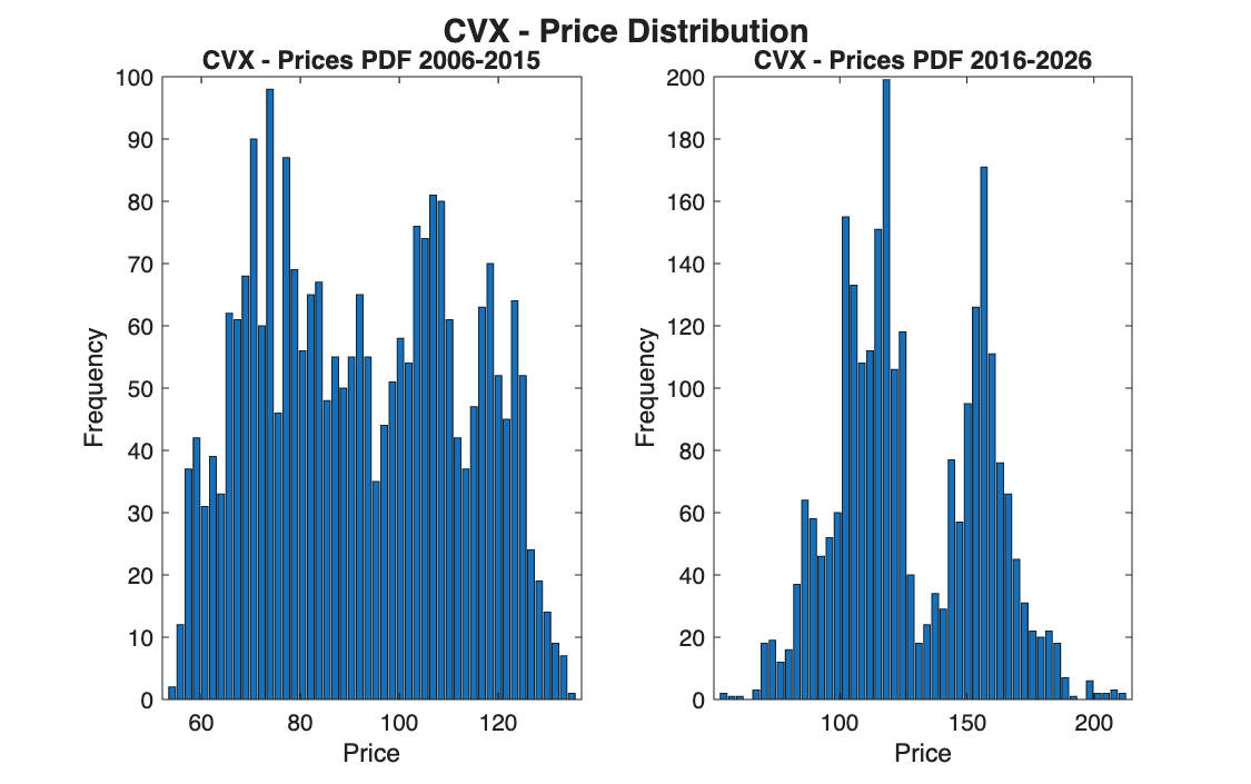
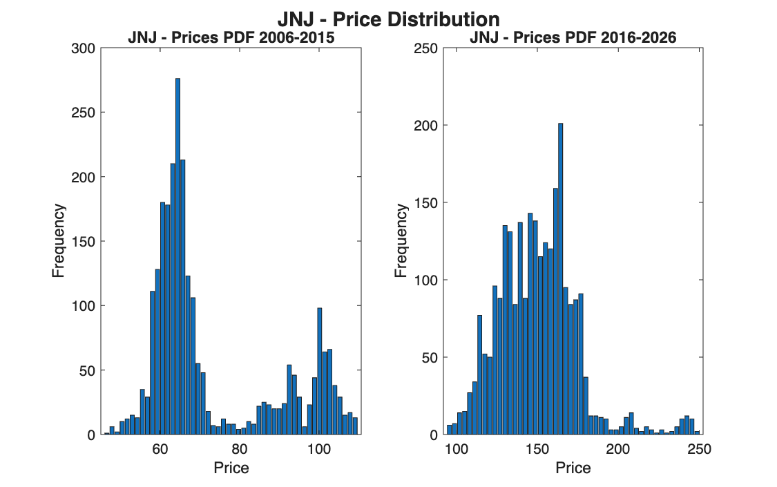
    % The visual evidence of non-stationarity is striking: in all 4 cases the
    % distributions cover completely different price ranges, with almost no
    % overlap.
    %
    % AAPL: the most extreme case. In 2006-2015 prices between $2 and $30; in
    %       2016-2026 between $40 and $280. The distribution moves by an order
    %       of magnitude.
    % JPM:  from bell-shaped ($20-$65) in P1 to bimodal ($50-$330) in P2.
    %       The two peaks of P2 reflect the pre- and post-Covid-19 phases.
    % CVX:  flat and wide distribution in P1 ($55-$135), typical of an energy
    %       stock. In P2 two separate clusters (2020 crash + recovery).
    % JNJ:  moves from $50-110 to $100-250, keeping a more regular shape —
    %       consistent with the defensive nature of the healthcare sector.


% 4.2 Summary statistics of the prices

    % Period 1
    [E_AAPL_p1, Var_AAPL_p1, Skew_AAPL_p1, Kurt_AAPL_p1] = F_es100(AAPL_p1);
    [E_JPM_p1,  Var_JPM_p1,  Skew_JPM_p1,  Kurt_JPM_p1]  = F_es100(JPM_p1);
    [E_CVX_p1,  Var_CVX_p1,  Skew_CVX_p1,  Kurt_CVX_p1]  = F_es100(CVX_p1);
    [E_JNJ_p1,  Var_JNJ_p1,  Skew_JNJ_p1,  Kurt_JNJ_p1]  = F_es100(JNJ_p1);

    % Period 2
    [E_AAPL_p2, Var_AAPL_p2, Skew_AAPL_p2, Kurt_AAPL_p2] = F_es100(AAPL_p2);
    [E_JPM_p2,  Var_JPM_p2,  Skew_JPM_p2,  Kurt_JPM_p2]  = F_es100(JPM_p2);
    [E_CVX_p2,  Var_CVX_p2,  Skew_CVX_p2,  Kurt_CVX_p2]  = F_es100(CVX_p2);
    [E_JNJ_p2,  Var_JNJ_p2,  Skew_JNJ_p2,  Kurt_JNJ_p2]  = F_es100(JNJ_p2);

    %              MEAN        VARIANCE     SKEWNESS    KURTOSIS
    % AAPL  P1:    13.04         81.14        0.57        2.12
    % AAPL  P2:   119.98       5675.50        0.29        1.80
    % JPM   P1:    45.99         96.93        0.29        2.81
    % JPM   P2:   143.99       4215.60        1.19        3.67
    % CVX   P1:    92.45        405.86        0.06        1.84
    % CVX   P2:   127.98        794.41        0.18        2.17
    % JNJ   P1:    72.81        254.63        0.95        2.37
    % JNJ   P2:   150.13        590.96        0.85        5.13
    %
    % Comment:
    % MEAN:     changes drastically for every stock. AAPL: from $13 to $120
    %           (+820%). A stationary process would have a stable mean.
    % VARIANCE: explodes in P2. AAPL: from 81 to 5676 (x70). Higher prices
    %           mean larger absolute swings.
    % SKEWNESS: changes sign or intensity — the shape of the distribution is
    %           not constant. JPM goes from 0.29 to 1.19 in the second period.
    % KURTOSIS: all values < 3 — prices have lighter tails than a Gaussian,
    %           the opposite of returns (see below).


% 4.3 PDF of the returns

    nbins_r = 100;

    figure(9)
    subplot(1,2,1); F_es99(AAPL_r1, nbins_r); title('AAPL - Returns PDF 2006-2015'); xlabel('Return'); ylabel('Frequency');
    subplot(1,2,2); F_es99(AAPL_r2, nbins_r); title('AAPL - Returns PDF 2016-2026'); xlabel('Return'); ylabel('Frequency');
    sgtitle('AAPL - Returns Distribution', 'FontSize', 14, 'FontWeight', 'bold');

    figure(10)
    subplot(1,2,1); F_es99(JPM_r1, nbins_r); title('JPM - Returns PDF 2006-2015'); xlabel('Return'); ylabel('Frequency');
    subplot(1,2,2); F_es99(JPM_r2, nbins_r); title('JPM - Returns PDF 2016-2026'); xlabel('Return'); ylabel('Frequency');
    sgtitle('JPM - Returns Distribution', 'FontSize', 14, 'FontWeight', 'bold');

    figure(11)
    subplot(1,2,1); F_es99(CVX_r1, nbins_r); title('CVX - Returns PDF 2006-2015'); xlabel('Return'); ylabel('Frequency');
    subplot(1,2,2); F_es99(CVX_r2, nbins_r); title('CVX - Returns PDF 2016-2026'); xlabel('Return'); ylabel('Frequency');
    sgtitle('CVX - Returns Distribution', 'FontSize', 14, 'FontWeight', 'bold');

    figure(12)
    subplot(1,2,1); F_es99(JNJ_r1, nbins_r); title('JNJ - Returns PDF 2006-2015'); xlabel('Return'); ylabel('Frequency');
    subplot(1,2,2); F_es99(JNJ_r2, nbins_r); title('JNJ - Returns PDF 2016-2026'); xlabel('Return'); ylabel('Frequency');
    sgtitle('JNJ - Returns Distribution', 'FontSize', 14, 'FontWeight', 'bold');

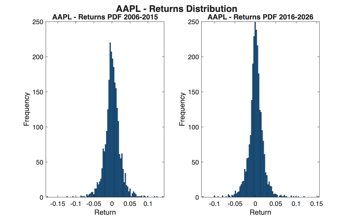
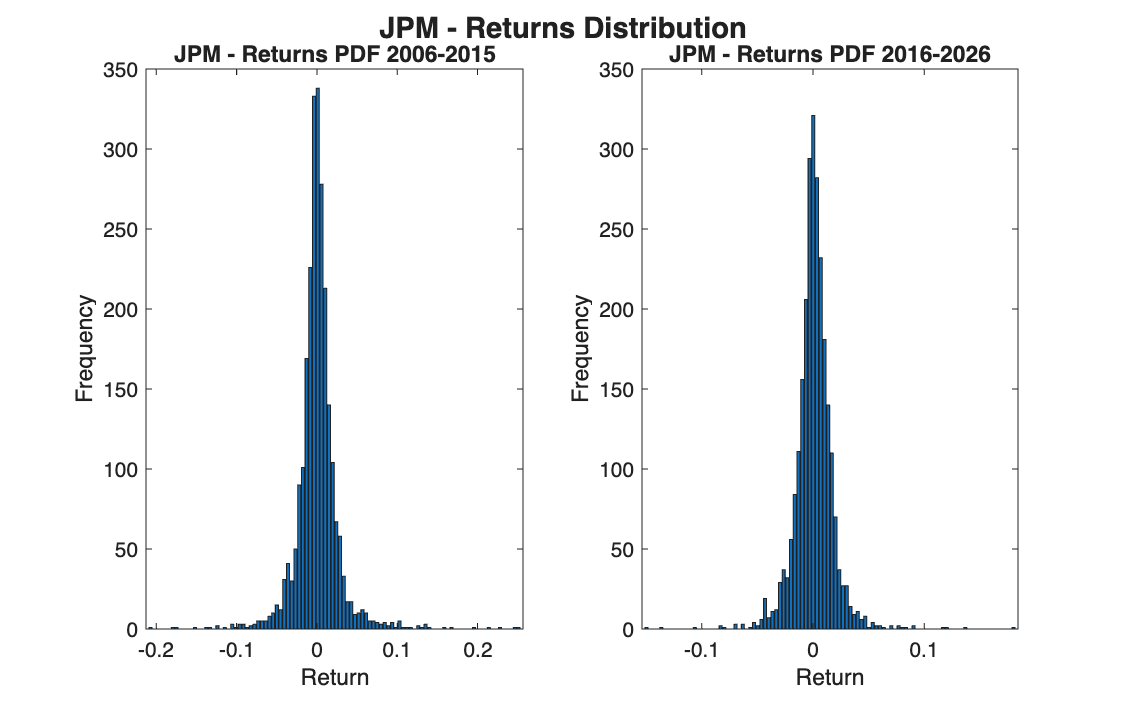
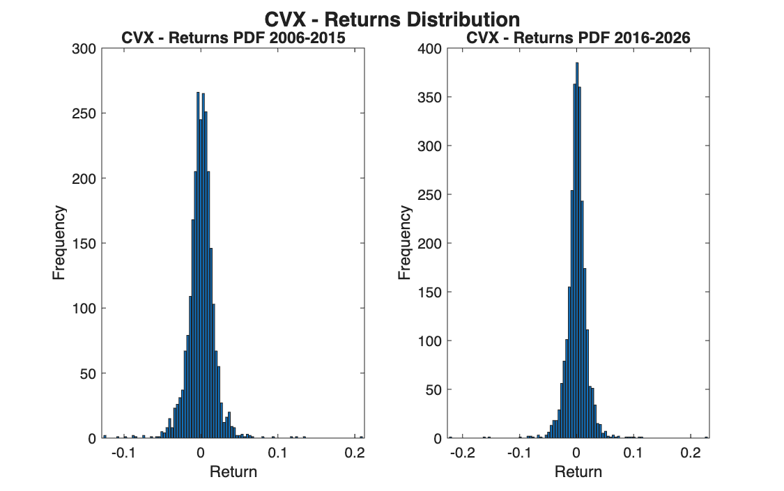
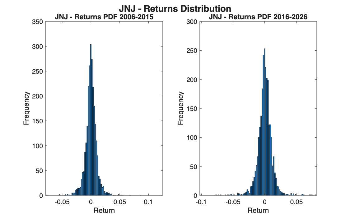
    % Results - PDF of the returns:
    % The contrast with prices is immediate: the distributions of the two
    % periods almost overlap for all 4 stocks. Same bell shape, same centre
    % around zero, same order of magnitude in the tails.
    %
    % AAPL: centred on zero, tails between -0.15 and +0.15.
    %       The shape is practically identical in the two periods.
    % JPM:  similar in the two periods. P1 shows slightly heavier tails
    %       because of the 2008 financial crisis.
    % CVX:  almost identical in shape and width, tails between -0.20 and +0.20.
    % JNJ:  the most stable stock — much narrower tails (+-0.08), the two
    %       distributions overlap almost perfectly.


% 4.4 Summary statistics of the returns

    % Period 1
    [E_AAPL_r1, Var_AAPL_r1, Skew_AAPL_r1, Kurt_AAPL_r1] = F_es100(AAPL_r1);
    [E_JPM_r1,  Var_JPM_r1,  Skew_JPM_r1,  Kurt_JPM_r1]  = F_es100(JPM_r1);
    [E_CVX_r1,  Var_CVX_r1,  Skew_CVX_r1,  Kurt_CVX_r1]  = F_es100(CVX_r1);
    [E_JNJ_r1,  Var_JNJ_r1,  Skew_JNJ_r1,  Kurt_JNJ_r1]  = F_es100(JNJ_r1);

    % Period 2
    [E_AAPL_r2, Var_AAPL_r2, Skew_AAPL_r2, Kurt_AAPL_r2] = F_es100(AAPL_r2);
    [E_JPM_r2,  Var_JPM_r2,  Skew_JPM_r2,  Kurt_JPM_r2]  = F_es100(JPM_r2);
    [E_CVX_r2,  Var_CVX_r2,  Skew_CVX_r2,  Kurt_CVX_r2]  = F_es100(CVX_r2);
    [E_JNJ_r2,  Var_JNJ_r2,  Skew_JNJ_r2,  Kurt_JNJ_r2]  = F_es100(JNJ_r2);

    %              MEAN (x1e-4)   VARIANCE (x1e-4)  SKEWNESS   KURTOSIS
    % AAPL  P1:      10.11            4.62            -0.07       8.33
    % AAPL  P2:       9.74            3.33             0.15       9.86
    % JPM   P1:       5.77            7.68             1.00      18.82
    % JPM   P2:       7.33            3.02             0.32      16.46
    % CVX   P1:       3.19            3.05             0.54      18.53
    % CVX   P2:       4.77            3.41            -0.31      27.03
    % JNJ   P1:       2.56            1.06             0.68      16.85
    % JNJ   P2:       4.03            1.34            -0.22      12.45
    %
    % Comment:
    % MEAN:     same order of magnitude in the two periods — no systematic
    %           drift. AAPL stays around 0.001 in both periods.
    % VARIANCE: same order of magnitude (1e-4) in both periods.
    %           JPM falls from 7.68 to 3.02: lower volatility after the 2008 crisis.
    % SKEWNESS: small values of varying sign — no systematic asymmetry.
    %           It changes sign between the periods for AAPL, CVX and JNJ.
    % KURTOSIS: all values >> 3 in both periods — persistent fat tails.
    %           Extreme events happen far more often than a Gaussian
    %           predicts. A property that is stable over time.
    %
    % Overall conclusion:
    % Prices are NOT stationary: mean, variance and shape change drastically
    % between the two periods for every stock.
    % Returns ARE (approximately) stationary: their distribution stays stable
    % over time. This is the fundamental reason why finance always works with
    % returns and not with prices.
function [xx, N] = F_es99(Y, nbins)

% This function computes an histogram of a PDF, given a vector of random outcomes

% inputs:   Y     = vector of random outcomes
%           nbins = number of bar for the histogram

% outputs:  xx = location of each bin
%           N  = number of elements in each bin

Ymin = min(Y); % smallest value of Y
Ymax = max(Y); % largest value of Y
               % together: the range the samples span

binc  = linspace(Ymin, Ymax, nbins); % nbins equally spaced points over [Ymin, Ymax]

[N, xx] = hist(Y, binc); % histogram with one bin centred on each point of binc

bar(xx, N); % bar creates a bar graph with one bar for each element in y

title('empirical probability density function');

end
function [E_x, Var_x, Skew_x, Kurt_x] = F_es100(x)

% Function computing several summary statistics

% Expected value
E_x   = mean(x);        % arithmetic mean
x_    = x - (E_x);      % deviations: how far each observation is from the mean

% Variance
Var_x = mean((x_).^2);  % the variance is the mean of the squared deviations
dev_x = sqrt(Var_x);    % standard deviation (square root of the variance)

% Skewness
Skew_x = mean((x_ ./ dev_x).^3); % deviations divided by the standard deviation (standardisation)
                                 % make the measure unit-free; then cube and average.

% Kurtosis
Kurt_x = mean((x_ ./ dev_x).^4); % same logic as the skewness, with the fourth power (always positive).
                                 % It measures how peaked the distribution is and how heavy its tails are.
                                 % A normal distribution has kurtosis = 3; higher values mean a sharper
                                 % peak and fat tails, lower values a flatter distribution.

end

% alternatively, MATLAB's built-in functions:
% kurtosis(x)
% skewness (x)
% var(x)
import numpy as np
import pandas as pd
import matplotlib.pyplot as plt
from scipy.stats import skew, kurtosis
from F_es99 import F_es99
from F_es100 import F_es100

np.set_printoptions(suppress=True)     # print numbers as 13.04, not 1.304e+01

# The stocks of exercise 119 are not in DowJones_price.xlsx: AAPL, JPM, CVX, JNJ are used.

# %% Point 1 - Import and returns

T = pd.read_excel("DowJones_price.xlsx")       # MATLAB: readtable("DowJones_price.xlsx")

# --- Prices ---
AAPL_prices = T['AAPL.OQ'].to_numpy()          # MATLAB: T{:, 'AAPL_OQ'}
                                               # (the column is called AAPL.OQ: MATLAB turns the dot into _)
JPM_prices  = T['JPM.N'].to_numpy()
CVX_prices  = T['CVX.N'].to_numpy()
JNJ_prices  = T['JNJ.N'].to_numpy()

# --- Linear returns ---
AAPL_returns = np.diff(AAPL_prices) / AAPL_prices[:-1]
JPM_returns  = np.diff(JPM_prices)  / JPM_prices[:-1]
CVX_returns  = np.diff(CVX_prices)  / CVX_prices[:-1]
JNJ_returns  = np.diff(JNJ_prices)  / JNJ_prices[:-1]

# --- Full returns matrix, saved to file ---
Returns = np.column_stack([AAPL_returns, JPM_returns, CVX_returns, JNJ_returns])
pd.DataFrame(Returns).to_excel('DowJones_returns.xlsx', index=False, header=False)   # MATLAB: writematrix

# %% Point 2 - Plot of the returns
plt.figure(1)
plt.plot(AAPL_returns)
plt.title('AAPL - Apple'); plt.ylabel('Linear Returns'); plt.xlabel('Days')
plt.figure(2)
plt.plot(JPM_returns)
plt.title('JPM - JP Morgan'); plt.ylabel('Linear Returns'); plt.xlabel('Days')
plt.figure(3)
plt.plot(CVX_returns)
plt.title('CVX - Chevron'); plt.ylabel('Linear Returns'); plt.xlabel('Days')
plt.figure(4)
plt.plot(JNJ_returns)
plt.title('JNJ - J&J'); plt.ylabel('Linear Returns'); plt.xlabel('Days')

# %% Point 3 - Descriptive statistics (one value per column = per asset)

Exp_returns = np.mean(Returns, axis=0)          # MATLAB: mean(Returns, 1)   (axis=0 = down the rows)
Std         = np.std(Returns, axis=0)           # MATLAB: std(Returns, 1)    (divides by N)
Skew        = skew(Returns, axis=0)             # MATLAB: skewness(Returns, 1)
Kurt        = kurtosis(Returns, axis=0, fisher=False)   # MATLAB: kurtosis(Returns, 1)   (normal = 3)
Sigma       = np.cov(Returns, rowvar=False)     # MATLAB: cov(Returns)   (rowvar=False: columns are the variables)

print("Exp_returns =", Exp_returns)
print("Std =", Std)
print("Skew =", Skew)
print("Kurt =", Kurt)

# %% Point 4 - Stationarity analysis
# Split: Period 1 = 2006-2015 (2513 obs) | Period 2 = 2016-2026 (2576 obs)

split   = 2513
split_r = split - 1                             # there is one return fewer than prices

# --- Split prices ---   (MATLAB: x(1:split) -> Python: x[:split];  x(split+1:end) -> x[split:])
AAPL_p1 = AAPL_prices[:split];   AAPL_p2 = AAPL_prices[split:]
JPM_p1 = JPM_prices[:split];    JPM_p2 = JPM_prices[split:]
CVX_p1 = CVX_prices[:split];    CVX_p2 = CVX_prices[split:]
JNJ_p1 = JNJ_prices[:split];    JNJ_p2 = JNJ_prices[split:]

# --- Split returns ---
AAPL_r1 = AAPL_returns[:split_r];   AAPL_r2 = AAPL_returns[split_r:]
JPM_r1 = JPM_returns[:split_r];    JPM_r2 = JPM_returns[split_r:]
CVX_r1 = CVX_returns[:split_r];    CVX_r2 = CVX_returns[split_r:]
JNJ_r1 = JNJ_returns[:split_r];    JNJ_r2 = JNJ_returns[split_r:]

# %% 4.1 PDF of the prices

nbins_p = 50

plt.figure(5)
plt.subplot(1, 2, 1); F_es99(AAPL_p1, nbins_p); plt.title('AAPL - Prices PDF 2006-2015'); plt.xlabel('Price'); plt.ylabel('Frequency')
plt.subplot(1, 2, 2); F_es99(AAPL_p2, nbins_p); plt.title('AAPL - Prices PDF 2016-2026'); plt.xlabel('Price'); plt.ylabel('Frequency')
plt.suptitle('AAPL - Price Distribution', fontsize=14, fontweight='bold')   # MATLAB: sgtitle

plt.figure(6)
plt.subplot(1, 2, 1); F_es99(JPM_p1, nbins_p); plt.title('JPM - Prices PDF 2006-2015'); plt.xlabel('Price'); plt.ylabel('Frequency')
plt.subplot(1, 2, 2); F_es99(JPM_p2, nbins_p); plt.title('JPM - Prices PDF 2016-2026'); plt.xlabel('Price'); plt.ylabel('Frequency')
plt.suptitle('JPM - Price Distribution', fontsize=14, fontweight='bold')   # MATLAB: sgtitle

plt.figure(7)
plt.subplot(1, 2, 1); F_es99(CVX_p1, nbins_p); plt.title('CVX - Prices PDF 2006-2015'); plt.xlabel('Price'); plt.ylabel('Frequency')
plt.subplot(1, 2, 2); F_es99(CVX_p2, nbins_p); plt.title('CVX - Prices PDF 2016-2026'); plt.xlabel('Price'); plt.ylabel('Frequency')
plt.suptitle('CVX - Price Distribution', fontsize=14, fontweight='bold')   # MATLAB: sgtitle

plt.figure(8)
plt.subplot(1, 2, 1); F_es99(JNJ_p1, nbins_p); plt.title('JNJ - Prices PDF 2006-2015'); plt.xlabel('Price'); plt.ylabel('Frequency')
plt.subplot(1, 2, 2); F_es99(JNJ_p2, nbins_p); plt.title('JNJ - Prices PDF 2016-2026'); plt.xlabel('Price'); plt.ylabel('Frequency')
plt.suptitle('JNJ - Price Distribution', fontsize=14, fontweight='bold')   # MATLAB: sgtitle

# %% 4.2 Summary statistics of the prices

E_AAPL_p1, Var_AAPL_p1, Skew_AAPL_p1, Kurt_AAPL_p1 = F_es100(AAPL_p1)
E_JPM_p1, Var_JPM_p1, Skew_JPM_p1, Kurt_JPM_p1 = F_es100(JPM_p1)
E_CVX_p1, Var_CVX_p1, Skew_CVX_p1, Kurt_CVX_p1 = F_es100(CVX_p1)
E_JNJ_p1, Var_JNJ_p1, Skew_JNJ_p1, Kurt_JNJ_p1 = F_es100(JNJ_p1)

E_AAPL_p2, Var_AAPL_p2, Skew_AAPL_p2, Kurt_AAPL_p2 = F_es100(AAPL_p2)
E_JPM_p2, Var_JPM_p2, Skew_JPM_p2, Kurt_JPM_p2 = F_es100(JPM_p2)
E_CVX_p2, Var_CVX_p2, Skew_CVX_p2, Kurt_CVX_p2 = F_es100(CVX_p2)
E_JNJ_p2, Var_JNJ_p2, Skew_JNJ_p2, Kurt_JNJ_p2 = F_es100(JNJ_p2)

print("prices (mean, variance, skewness, kurtosis), period 1 and period 2:")
print("AAPL", np.round([E_AAPL_p1, Var_AAPL_p1, Skew_AAPL_p1, Kurt_AAPL_p1], 2), np.round([E_AAPL_p2, Var_AAPL_p2, Skew_AAPL_p2, Kurt_AAPL_p2], 2))
print("JPM ", np.round([E_JPM_p1, Var_JPM_p1, Skew_JPM_p1, Kurt_JPM_p1], 2), np.round([E_JPM_p2, Var_JPM_p2, Skew_JPM_p2, Kurt_JPM_p2], 2))
print("CVX ", np.round([E_CVX_p1, Var_CVX_p1, Skew_CVX_p1, Kurt_CVX_p1], 2), np.round([E_CVX_p2, Var_CVX_p2, Skew_CVX_p2, Kurt_CVX_p2], 2))
print("JNJ ", np.round([E_JNJ_p1, Var_JNJ_p1, Skew_JNJ_p1, Kurt_JNJ_p1], 2), np.round([E_JNJ_p2, Var_JNJ_p2, Skew_JNJ_p2, Kurt_JNJ_p2], 2))

# %% 4.3 PDF of the returns

nbins_r = 100

plt.figure(9)
plt.subplot(1, 2, 1); F_es99(AAPL_r1, nbins_r); plt.title('AAPL - Returns PDF 2006-2015'); plt.xlabel('Return'); plt.ylabel('Frequency')
plt.subplot(1, 2, 2); F_es99(AAPL_r2, nbins_r); plt.title('AAPL - Returns PDF 2016-2026'); plt.xlabel('Return'); plt.ylabel('Frequency')
plt.suptitle('AAPL - Returns Distribution', fontsize=14, fontweight='bold')

plt.figure(10)
plt.subplot(1, 2, 1); F_es99(JPM_r1, nbins_r); plt.title('JPM - Returns PDF 2006-2015'); plt.xlabel('Return'); plt.ylabel('Frequency')
plt.subplot(1, 2, 2); F_es99(JPM_r2, nbins_r); plt.title('JPM - Returns PDF 2016-2026'); plt.xlabel('Return'); plt.ylabel('Frequency')
plt.suptitle('JPM - Returns Distribution', fontsize=14, fontweight='bold')

plt.figure(11)
plt.subplot(1, 2, 1); F_es99(CVX_r1, nbins_r); plt.title('CVX - Returns PDF 2006-2015'); plt.xlabel('Return'); plt.ylabel('Frequency')
plt.subplot(1, 2, 2); F_es99(CVX_r2, nbins_r); plt.title('CVX - Returns PDF 2016-2026'); plt.xlabel('Return'); plt.ylabel('Frequency')
plt.suptitle('CVX - Returns Distribution', fontsize=14, fontweight='bold')

plt.figure(12)
plt.subplot(1, 2, 1); F_es99(JNJ_r1, nbins_r); plt.title('JNJ - Returns PDF 2006-2015'); plt.xlabel('Return'); plt.ylabel('Frequency')
plt.subplot(1, 2, 2); F_es99(JNJ_r2, nbins_r); plt.title('JNJ - Returns PDF 2016-2026'); plt.xlabel('Return'); plt.ylabel('Frequency')
plt.suptitle('JNJ - Returns Distribution', fontsize=14, fontweight='bold')

# %% 4.4 Summary statistics of the returns

E_AAPL_r1, Var_AAPL_r1, Skew_AAPL_r1, Kurt_AAPL_r1 = F_es100(AAPL_r1)
E_JPM_r1, Var_JPM_r1, Skew_JPM_r1, Kurt_JPM_r1 = F_es100(JPM_r1)
E_CVX_r1, Var_CVX_r1, Skew_CVX_r1, Kurt_CVX_r1 = F_es100(CVX_r1)
E_JNJ_r1, Var_JNJ_r1, Skew_JNJ_r1, Kurt_JNJ_r1 = F_es100(JNJ_r1)

E_AAPL_r2, Var_AAPL_r2, Skew_AAPL_r2, Kurt_AAPL_r2 = F_es100(AAPL_r2)
E_JPM_r2, Var_JPM_r2, Skew_JPM_r2, Kurt_JPM_r2 = F_es100(JPM_r2)
E_CVX_r2, Var_CVX_r2, Skew_CVX_r2, Kurt_CVX_r2 = F_es100(CVX_r2)
E_JNJ_r2, Var_JNJ_r2, Skew_JNJ_r2, Kurt_JNJ_r2 = F_es100(JNJ_r2)

print("returns (mean x1e-4, variance x1e-4, skewness, kurtosis), period 1 and period 2:")
print("AAPL", np.round([E_AAPL_r1*1e4, Var_AAPL_r1*1e4, Skew_AAPL_r1, Kurt_AAPL_r1], 2), np.round([E_AAPL_r2*1e4, Var_AAPL_r2*1e4, Skew_AAPL_r2, Kurt_AAPL_r2], 2))
print("JPM ", np.round([E_JPM_r1*1e4, Var_JPM_r1*1e4, Skew_JPM_r1, Kurt_JPM_r1], 2), np.round([E_JPM_r2*1e4, Var_JPM_r2*1e4, Skew_JPM_r2, Kurt_JPM_r2], 2))
print("CVX ", np.round([E_CVX_r1*1e4, Var_CVX_r1*1e4, Skew_CVX_r1, Kurt_CVX_r1], 2), np.round([E_CVX_r2*1e4, Var_CVX_r2*1e4, Skew_CVX_r2, Kurt_CVX_r2], 2))
print("JNJ ", np.round([E_JNJ_r1*1e4, Var_JNJ_r1*1e4, Skew_JNJ_r1, Kurt_JNJ_r1], 2), np.round([E_JNJ_r2*1e4, Var_JNJ_r2*1e4, Skew_JNJ_r2, Kurt_JNJ_r2], 2))

plt.show()

# Conclusion: prices are not stationary (mean, variance and shape change between the
# periods); returns are approximately stationary, with persistent fat tails.
import numpy as np


def F_es100(x):
    # summary statistics: mean, variance, skewness, kurtosis

    E_x = np.mean(x)                    # expected value
    x_ = x - E_x                        # deviations from the mean

    Var_x = np.mean(x_**2)              # variance = mean of the squared deviations
    dev_x = np.sqrt(Var_x)              # standard deviation

    Skew_x = np.mean((x_ / dev_x)**3)   # skewness: standardised deviations, cubed, averaged
    Kurt_x = np.mean((x_ / dev_x)**4)   # kurtosis: same, fourth power (normal = 3)

    return E_x, Var_x, Skew_x, Kurt_x
import matplotlib.pyplot as plt


def F_es99(Y, nbins):
    # Histogram of a pdf, given a vector of random outcomes
    # inputs:   Y     = vector of random outcomes
    #           nbins = number of bars
    # outputs:  xx = location (centre) of each bar
    #           N  = number of elements in each bar

    N, edges, bars = plt.hist(Y, nbins)     # MATLAB: [N, xx] = hist(Y, binc); bar(xx, N)
    xx = (edges[:-1] + edges[1:]) / 2       # centre of each bar
    # (MATLAB's hist puts the centres of the first and last bar on min(Y) and max(Y);
    #  plt.hist puts the edges there, so the bars are slightly different)

    plt.title('empirical probability density function')
    return xx, N
Results
Full sample: daily returns
| AAPL | JPM | CVX | JNJ | |
|---|---|---|---|---|
| Mean | 0.110% | 0.066% | 0.040% | 0.033% |
| Standard deviation | 1.99% | 2.31% | 1.80% | 1.10% |
| Skewness | 0.02 | 0.92 | 0.08 | 0.15 |
| Kurtosis | 9.1 | 22.0 | 23.4 | 14.3 |
Correlations range from 0.31 (AAPL–JNJ) to 0.51 (JPM–CVX).
Prices: Period 1 against Period 2
| Mean | Variance | Skewness | Kurtosis | |
|---|---|---|---|---|
| AAPL | 13.04 → 119.98 | 81 → 5,675 | 0.57 → 0.29 | 2.12 → 1.80 |
| JPM | 45.99 → 143.99 | 97 → 4,216 | 0.29 → 1.19 | 2.81 → 3.67 |
| CVX | 92.45 → 127.98 | 406 → 794 | 0.06 → 0.18 | 1.84 → 2.17 |
| JNJ | 72.81 → 150.13 | 255 → 591 | 0.95 → 0.85 | 2.37 → 5.13 |
Returns: Period 1 against Period 2
Mean and variance in units of \(10^{-4}\).
| Mean | Variance | Skewness | Kurtosis | |
|---|---|---|---|---|
| AAPL | 11.43 → 10.49 | 4.62 → 3.33 | −0.07 → 0.15 | 8.33 → 9.86 |
| JPM | 5.77 → 7.33 | 7.68 → 3.02 | 1.00 → 0.32 | 18.82 → 16.46 |
| CVX | 3.19 → 4.77 | 3.05 → 3.41 | 0.54 → −0.31 | 18.53 → 27.03 |
| JNJ | 2.56 → 4.03 | 1.06 → 1.34 | 0.68 → −0.22 | 16.85 → 12.45 |
Two corrections to the comments in the code
The results table written in the code's comments matches the computation in every cell but one: the mean daily return of AAPL is 11.43 and 10.49 (\(\times 10^{-4}\)), not 10.11 and 9.74. The conclusion does not change.
In Point 3, the comment says the second argument of std, skewness and kurtosis is
the dimension, as for mean(Returns, 1). For those three functions it is a
normalisation flag instead: std(Returns, 1) divides by \(N\) rather than \(N - 1\). The
statistics are still computed column by column, and with 5,000 observations the
difference is invisible, but the reason in the comment is not the right one.
Takeaways
- Prices are not stationary. Their mean, variance and shape change completely between the two periods: AAPL's average price rises nine-fold and its variance seventy-fold.
- Returns are approximately stationary. Same centre, same order of magnitude of variance, similar shape in both periods. This is why models are built on returns.
- Fat tails are the stable feature. Kurtosis is far above 3 in both periods for every stock: extreme days happen much more often than a normal distribution predicts, and they keep happening.