Value at Risk and Conditional VaR by simulation¶

Course exercises 137–138 · Part II

Problem¶

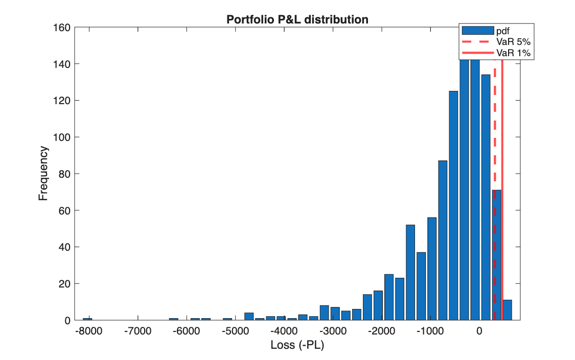
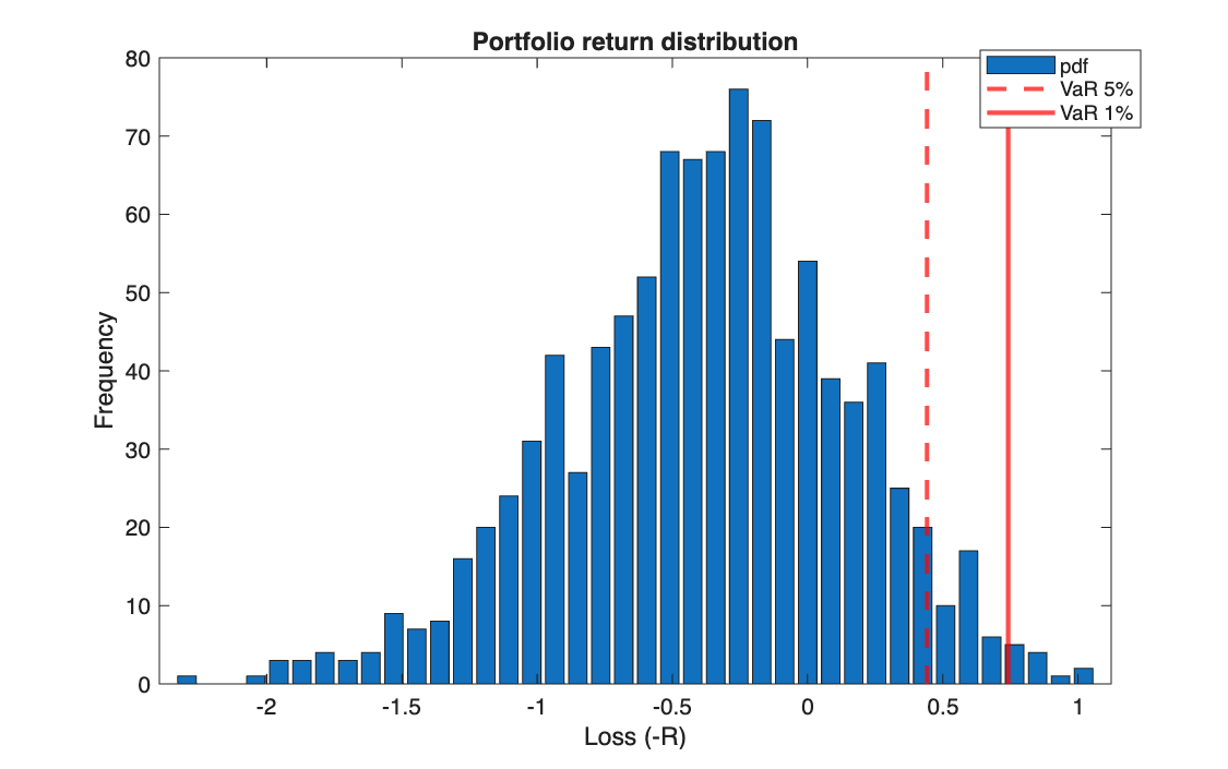
A portfolio of five stocks is worth 900 today. Simulate 1,000 scenarios of log-normal prices at the horizon, compute the profit and loss distribution, and estimate its Value at Risk at 5% and 1% (exercise 137) and its Conditional Value at Risk at 5% (exercise 138).

Method¶

Prices at the horizon are \(P_T = P_0\, e^{R}\) with \(R \sim \mathcal{N}(0, 1)\) for each stock, and \(PL = V_T - V_0\). With the \(m\) simulated P&L values sorted from the worst:

\[ \text{VaR}_\varepsilon = -PL_{(k)}, \qquad \text{CVaR}_\varepsilon = -\frac{1}{k}\sum_{i=1}^{k} PL_{(i)}, \qquad k \approx \varepsilon\, m \]

VaR is the loss exceeded only in the worst \(\varepsilon\) of scenarios; CVaR is the average loss in those scenarios.

Code¶

MATLABPython

S_exercise_137.mS_exercise_138.mF_Empirical_pdf.m

clear all, clc

%% 1

n = 5;   m = 1000;

P0 = [7 9 24 19 15];        % current prices
q  = [20 20 10 10 10];      % allocation (number of shares)
V0 = q * P0';               % initial portfolio value

R   = randn(m, n);          % simulated returns (standard normal)
P_T = P0 .* exp(R);         % future prices (log-normal): P_T = P0*e^R
V_T = P_T * q';             % future portfolio values (m x 1)

PL_T = V_T - V0;            % Profit & Loss
R_T  = log(V_T / V0);       % future portfolio return

save('PortPLandRet.mat', 'PL_T', 'R_T');

%% 2

PL_sort = sort(PL_T);       % increasing order: the first ones are the worst losses
RT_sort = sort(R_T);

% epsilon = 0.05
N5 = floor(0.05 * m) + 1;
VaR_PL_5 = -PL_sort(N5)
VaR_RT_5 = -RT_sort(N5)

% epsilon = 0.01
N1 = floor(0.01 * m) + 1;
VaR_PL_1 = -PL_sort(N1)
VaR_RT_1 = -RT_sort(N1)

%% 3

nbins = 40;

figure(1)
F_Empirical_pdf(-PL_T, nbins)
hold on
xline(VaR_PL_5, '--r', 'LineWidth', 2)
xline(VaR_PL_1, '-r',  'LineWidth', 2)
xlabel('Loss (-PL)'); ylabel('Frequency'); title('Portfolio P&L distribution')
legend('pdf', 'VaR 5%', 'VaR 1%')

figure(2)
F_Empirical_pdf(-R_T, nbins)
hold on
xline(VaR_RT_5, '--r', 'LineWidth', 2)
xline(VaR_RT_1, '-r',  'LineWidth', 2)
xlabel('Loss (-R)'); ylabel('Frequency'); title('Portfolio return distribution')
legend('pdf', 'VaR 5%', 'VaR 1%')

clear all, clc

% Point 1

    % Parameters
    n = 5;
    m = 1000;
    epsilon = 0.05;
    P0 = [7 9 24 19 15];
    q  = [20 20 10 10 10];
    V0 = q * P0';

    % Simulation
    R   = randn(m, n);
    P_T = repmat(P0, m, 1) .* exp(R);
    V_T = P_T * q';

    % P&L
    PL_T = V_T - V0;
    R_T  = log(V_T / V0);

    % Risk Measures
    PL_T_sort = sort(PL_T);
    Nepsilon  = round(epsilon * m); % round, because when epsilon*m is not an integer
                                    % the quantile index must still point to an element

    Q_PL_T  = PL_T_sort(Nepsilon);

    VaR_PL  = -Q_PL_T
    CVaR_PL = -mean(PL_T_sort(1:Nepsilon))

function [Emp_pdf] = F_Empirical_pdf(y, nbins)

y_min = min(y);

Y_max = max(y);

bins = linspace(y_min, Y_max, nbins);

[counts,centers] = hist(y , bins);

bar(centers, counts);

end

S_exercise_137.pyS_exercise_138.pyF_Empirical_pdf.py

import numpy as np
import matplotlib.pyplot as plt
from scipy.io import savemat
from F_Empirical_pdf import F_Empirical_pdf

# %% 1
n = 5
m = 1000

P0 = np.array([7, 9, 24, 19, 15])       # current prices
q = np.array([20, 20, 10, 10, 10])      # allocation (number of shares)
V0 = q @ P0                             # initial portfolio value

R = np.random.randn(m, n)               # simulated returns (standard normal)
P_T = P0 * np.exp(R)                    # future prices (log-normal): P_T = P0*e^R   (P0 is applied to every row)
V_T = P_T @ q                           # future portfolio values

PL_T = V_T - V0                         # Profit & Loss
R_T = np.log(V_T / V0)                  # future portfolio return

savemat('PortPLandRet.mat', {'PL_T': PL_T, 'R_T': R_T})

# %% 2
PL_sort = np.sort(PL_T)                 # increasing order: the first ones are the worst losses
RT_sort = np.sort(R_T)

# epsilon = 0.05
N5 = int(np.floor(0.05 * m)) + 1        # position in MATLAB numbering (51)
VaR_PL_5 = -PL_sort[N5 - 1]             # -1: Python counts from 0
VaR_RT_5 = -RT_sort[N5 - 1]
print("VaR_PL_5 =", VaR_PL_5, " VaR_RT_5 =", VaR_RT_5)

# epsilon = 0.01
N1 = int(np.floor(0.01 * m)) + 1
VaR_PL_1 = -PL_sort[N1 - 1]
VaR_RT_1 = -RT_sort[N1 - 1]
print("VaR_PL_1 =", VaR_PL_1, " VaR_RT_1 =", VaR_RT_1)

# %% 3
nbins = 40

plt.figure(1)
F_Empirical_pdf(-PL_T, nbins)
plt.axvline(VaR_PL_5, color='r', linestyle='--', linewidth=2, label='VaR 5%')   # MATLAB: xline
plt.axvline(VaR_PL_1, color='r', linestyle='-', linewidth=2, label='VaR 1%')
plt.xlabel('Loss (-PL)'); plt.ylabel('Frequency'); plt.title('Portfolio P&L distribution')
plt.legend()                            # shows the labels given above

plt.figure(2)
F_Empirical_pdf(-R_T, nbins)
plt.axvline(VaR_RT_5, color='r', linestyle='--', linewidth=2, label='VaR 5%')
plt.axvline(VaR_RT_1, color='r', linestyle='-', linewidth=2, label='VaR 1%')
plt.xlabel('Loss (-R)'); plt.ylabel('Frequency'); plt.title('Portfolio return distribution')
plt.legend()                            # shows the labels given above
plt.show()

import numpy as np

# %% Point 1

# Parameters
n = 5
m = 1000
epsilon = 0.05
P0 = np.array([7, 9, 24, 19, 15])
q = np.array([20, 20, 10, 10, 10])
V0 = q @ P0

# Simulation
R = np.random.randn(m, n)
P_T = np.tile(P0, (m, 1)) * np.exp(R)   # MATLAB: repmat(P0, m, 1) .* exp(R)
V_T = P_T @ q

# P&L
PL_T = V_T - V0
R_T = np.log(V_T / V0)

# Risk Measures
PL_T_sort = np.sort(PL_T)
Nepsilon = round(epsilon * m)           # 50: the quantile index must point to an element

Q_PL_T = PL_T_sort[Nepsilon - 1]        # MATLAB: PL_T_sort(Nepsilon)   (-1: Python counts from 0)

VaR_PL = -Q_PL_T
CVaR_PL = -np.mean(PL_T_sort[:Nepsilon])   # MATLAB: mean(PL_T_sort(1:Nepsilon))
print("VaR_PL =", VaR_PL)
print("CVaR_PL =", CVaR_PL)

import matplotlib.pyplot as plt


def F_Empirical_pdf(y, nbins):
    # histogram of the sample y with nbins bars
    counts, edges, bars = plt.hist(y, nbins)    # MATLAB: [counts, centers] = hist(y, bins); bar(centers, counts)
    return counts

Results¶

Both scripts draw the same 1,000 scenarios (random seed 0 when generating this page).

	5%	1%
VaR on P&L (exercise 137)	321.34	471.58
VaR on log return (exercise 137)	0.442	0.742
VaR on P&L (exercise 138)	322.88
CVaR on P&L (exercise 138)	415.71

P&LReturn

Distribution of the simulated losses with the two VaR levels

Distribution of the simulated return losses with the two VaR levels

Takeaways¶

On the same scenarios, the two scripts give two different 5% VaRs (321.34 and 322.88) because they pick different order statistics: the 51^st worst loss (floor(0.05*m) + 1) against the 50^th (round(0.05*m)). With a finite sample, the quantile convention is part of the definition.
CVaR is always at least as large as VaR, because it averages the losses beyond it: here 415.71 against 322.88.
With log-normal prices the loss is capped at the portfolio value (900), while gains are unbounded: the distribution is strongly asymmetric, which is why a normal approximation of the P&L would be poor.