Empirical distributions: CDF, histogram and moments¶

Course exercises 95, 99, 100 · Part II

Problem¶

Build the three basic tools for describing a random variable from data, each as a reusable function: the empirical cumulative distribution function of a discrete variable (exercise 95), the histogram of a sample as an estimate of its density (exercise 99), and the first four moments (exercise 100). The second and third are tested on standard normal samples.

Method¶

For a discrete variable with values \(x_i\) and probabilities \(p_i\), the CDF sums the probabilities of the values up to \(x\), so the values must be sorted first:

\[ F_X(x) = \sum_{x_i \le x} p_i \]

The histogram splits the range \([\min y, \max y]\) into equally spaced bins and counts the observations in each. The moments, with \(\bar{x}\) the mean and \(s\) the standard deviation:

\[ \bar{x} = \frac{1}{n}\sum x_i, \quad s^2 = \frac{1}{n}\sum (x_i - \bar{x})^2, \quad \text{skew} = \frac{1}{n}\sum \Big(\frac{x_i - \bar{x}}{s}\Big)^3, \quad \text{kurt} = \frac{1}{n}\sum \Big(\frac{x_i - \bar{x}}{s}\Big)^4 \]

Code¶

MATLABPython

S_exercise_95.mF_es95.mS_exercise_99.mS_exercise_100.m

clear all, clc

% detailed explanation in F_es95

% Point 1
    x = [ 2 4 1 5];
    p = [ 1/4 1/16 1/2 3/16];
    % check that the probabilities sum to 1: sum(p)

    [x_sort, Emp_cdf] = F_es95(x, p)

function [x_sort, Emp_cdf] = F_es95(x, p)

% The CDF (Cumulative Distribution Function) must be computed in increasing
% order of x: otherwise cumsum would add up the probabilities in the wrong
% order and the result would be meaningless.

% inputs:    x := random vector (values of the random variable)
%            p := probabilities linked to each element of x
% outputs:   x_sort := vector of the sorted random variables x
%            Emp_cdf := vector of the cumulative probabilities associated with x_sort

[x_sort, Ind_sort] = sort(x);   % example: x = [5, 2, 8]
                                % x_sort    = [2, 5, 8]
                                % Ind_sort  = [2, 1, 3]   (original position of each element)

p_sort = p(Ind_sort);           % reorder the probabilities to follow x_sort (otherwise they would be attached to the wrong values)

Emp_cdf = cumsum(p_sort);       % cumulative sum of the probabilities

stairs(x_sort, Emp_cdf, 'LineWidth', 2)   % plotting the CDF (stairs, because an empirical CDF is piecewise constant)
title('Empirical Cumulative Distribution Function')
xlabel('x')
ylabel('F_X(x)')
% figure

end

clear all, clc

% Point 1
    n = 100000;
    y = randn(n, 1);
    nbins = 4000;
    [xx, N] = F_es99(y, nbins);


function [xx, N] = F_es99(Y, nbins)

% This function computes an histogram of a pdf, given a vector of random outcomes

% inputs:   Y     = vector of random outcomes
%           nbins = number of bar for the histogram

% outputs:  xx = location of each bin
%           N  = number of elements in each bin

Ymin = min(Y); % smallest value of Y
Ymax = max(Y); % largest value of Y
               % together: the range the samples span

binc  = linspace(Ymin, Ymax, nbins); % nbins equally spaced points over [Ymin, Ymax]

[N, xx] = hist(Y, binc); % histogram with one bin centred on each point of binc

bar(xx, N); % bar creates a bar graph with one bar for each element in y

title('empirical probability density function');

end

%
% Goal: answer the question "given a set of random values, how often do
% certain values occur?". The answer is the empirical distribution, shown
% as a histogram.
%
% THE LOGIC IN THREE STEPS:
%
% 1) FIND THE BOUNDARIES
%    min(Y) and max(Y) give the interval that contains all the data.
%    A space cannot be split into equal parts before knowing how big it is.
%
% 2) SPLIT THE SPACE INTO EQUAL PARTS
%    linspace creates 'nbins' equally spaced centres between Ymin and Ymax.
%    Each centre defines a "bin" that collects the values of Y close to it.
%    More bins = more resolution; fewer bins = a coarser view.
%
% 3) COUNT AND DRAW
%    hist assigns each value of Y to the nearest bin and counts them.
%    bar turns the counts into a bar chart:
%    tall bars = frequent values, short bars = rare values.
%
% NOTE: the chart shows the *empirical* distribution, the one actually
% observed in the data, not the theoretical one. With many samples in Y
% the two converge (law of large numbers).

clear all, clc

% Point 1
    n = 1000000;
    x = randn(n, 1);

    [E_x, Var_x, Skew_x, Kurt_x] = F_es100(x)


function [E_x, Var_x, Skew_x, Kurt_x] = F_es100(x)

% Function computing several summary statistics

% Expected value
E_x   = mean(x);        % arithmetic mean
x_    = x - (E_x);      % deviations: how far each observation is from the mean

% Variance
Var_x = mean((x_).^2);  % the variance is the mean of the squared deviations
dev_x = sqrt(Var_x);    % standard deviation (square root of the variance)

% Skewness
Skew_x = mean((x_ ./ dev_x).^3); % deviations divided by the standard deviation (standardisation)
                                 % make the measure unit-free; then cube and average.

% Kurtosis
Kurt_x = mean((x_ ./ dev_x).^4); % same logic as the skewness, with the fourth power (always positive).
                                 % It measures how peaked the distribution is and how heavy its tails are.
                                 % A normal distribution has kurtosis = 3; higher values mean a sharper
                                 % peak and fat tails, lower values a flatter distribution.

end

% alternatively, MATLAB's built-in functions:
% kurtosis(x)
% skewness (x)
% var(x)

S_exercise_95.pyS_exercise_99.pyS_exercise_100.pyF_es95.py

import matplotlib.pyplot as plt
from F_es95 import F_es95

# %% Point 1
x = [2, 4, 1, 5]
p = [1/4, 1/16, 1/2, 3/16]
# check that the probabilities sum to 1: sum(p)

x_sort, Emp_cdf = F_es95(x, p)
print("x_sort =", x_sort)
print("Emp_cdf =", Emp_cdf)

plt.show()

import numpy as np
import matplotlib.pyplot as plt


# %% function F_es99

def F_es99(Y, nbins):
    # Histogram of a pdf, given a vector of random outcomes
    # inputs:   Y     = vector of random outcomes
    #           nbins = number of bars
    # outputs:  xx = location (centre) of each bar
    #           N  = number of elements in each bar

    N, edges, bars = plt.hist(Y, nbins)     # MATLAB: [N, xx] = hist(Y, binc); bar(xx, N)
    xx = (edges[:-1] + edges[1:]) / 2       # centre of each bar
    # (MATLAB's hist puts the centres of the first and last bar on min(Y) and max(Y);
    #  plt.hist puts the edges there, so the bars are slightly different)

    plt.title('empirical probability density function')
    return xx, N


# %% Point 1
n = 100000
y = np.random.randn(n)                  # MATLAB: randn(n, 1)
nbins = 4000
xx, N = F_es99(y, nbins)

plt.show()

# The logic in three steps:
# 1) find the boundaries: min and max of the data
# 2) split that space into nbins equal parts
# 3) count the values in each part and draw the bars
# The chart shows the empirical distribution; with many samples it converges
# to the theoretical one (law of large numbers).

import numpy as np


# %% function F_es100

def F_es100(x):
    # summary statistics: mean, variance, skewness, kurtosis

    E_x = np.mean(x)                    # expected value
    x_ = x - E_x                        # deviations from the mean

    Var_x = np.mean(x_**2)              # variance = mean of the squared deviations
    dev_x = np.sqrt(Var_x)              # standard deviation

    Skew_x = np.mean((x_ / dev_x)**3)   # skewness: standardised deviations, cubed, averaged
    Kurt_x = np.mean((x_ / dev_x)**4)   # kurtosis: same, fourth power (normal = 3)

    return E_x, Var_x, Skew_x, Kurt_x


# %% Point 1
n = 1000000
x = np.random.randn(n)

E_x, Var_x, Skew_x, Kurt_x = F_es100(x)
print("E_x =", E_x)
print("Var_x =", Var_x)
print("Skew_x =", Skew_x)
print("Kurt_x =", Kurt_x)

# alternatively, ready-made functions:
# np.var(x), scipy.stats.skew(x), scipy.stats.kurtosis(x, fisher=False)

import numpy as np
import matplotlib.pyplot as plt


def F_es95(x, p):
    # The CDF must be computed in increasing order of x: sort first.
    # inputs:    x := values of the random variable
    #            p := probabilities linked to each element of x
    # outputs:   x_sort  := x sorted in increasing order
    #            Emp_cdf := cumulative probabilities associated with x_sort

    x = np.array(x)
    p = np.array(p)

    Ind_sort = np.argsort(x)            # MATLAB: [x_sort, Ind_sort] = sort(x)   (argsort gives the positions)
    x_sort = x[Ind_sort]

    p_sort = p[Ind_sort]                # reorder the probabilities to follow x_sort

    Emp_cdf = np.cumsum(p_sort)         # cumulative sum of the probabilities

    plt.step(x_sort, Emp_cdf, where='post', linewidth=2)   # MATLAB: stairs (a CDF is piecewise constant)
    plt.title('Empirical Cumulative Distribution Function')
    plt.xlabel('x')
    plt.ylabel('F_X(x)')

    return x_sort, Emp_cdf

Results¶

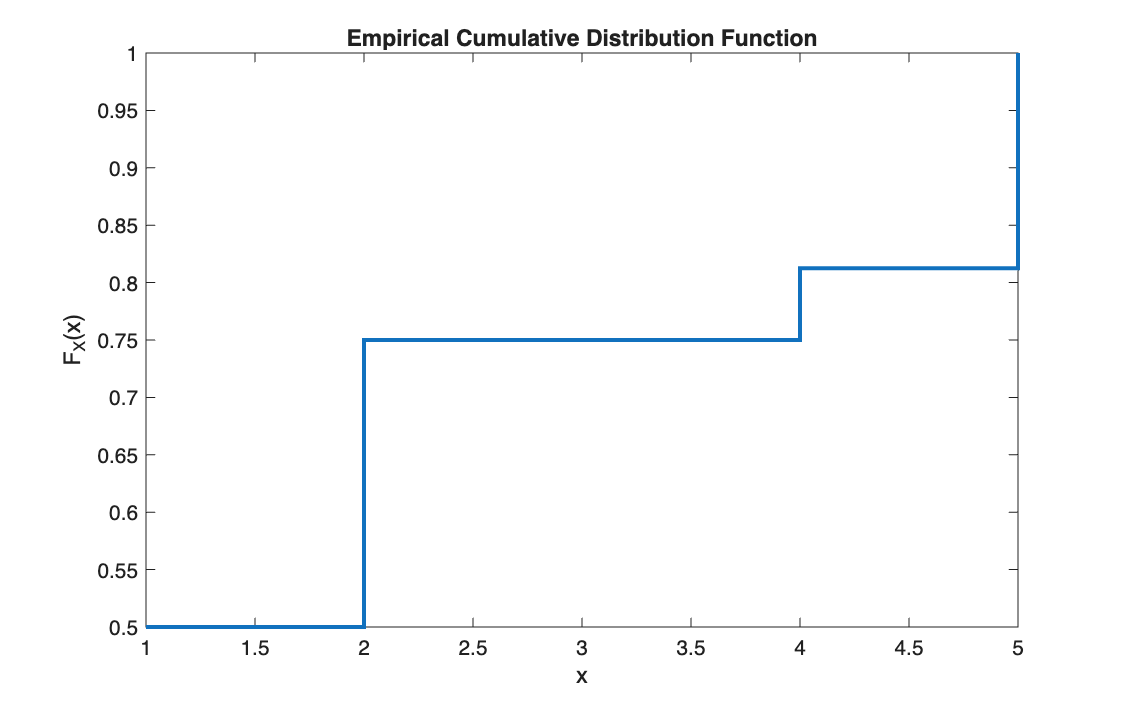
CDF (exercise 95). Values \(x = (2, 4, 1, 5)\) with probabilities \((1/4, 1/16, 1/2, 3/16)\): sorted, the CDF is 0.5, 0.75, 0.8125, 1.

Empirical CDFHistogram of 100,000 normal draws

Empirical CDF of the discrete variable

Histogram of 100,000 standard normal draws with 4,000 bins

Moments (exercise 100). On one million standard normal draws:

	Sample	Theory
Mean	0.0009	0
Variance	0.9994	1
Skewness	0.0003	0
Kurtosis	3.0042	3

Takeaways¶

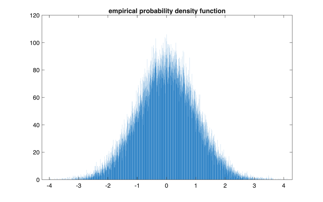
An empirical CDF is a step function: stairs, not plot.
The number of bins is a choice: 4,000 bins on 100,000 draws gives about 25 observations per bin, enough to see the bell shape but visibly noisy.
Kurtosis is measured against 3, the value of the normal distribution: it is the reference used throughout the rest of this part.