How much risk diversification removes
Problem
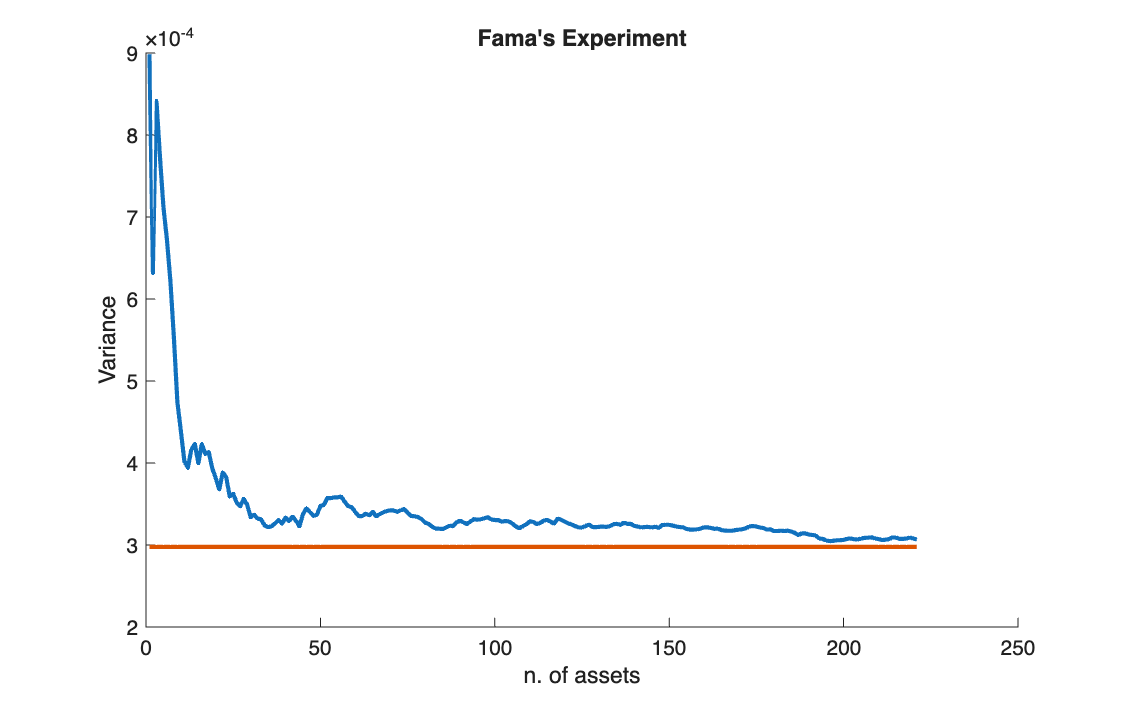
With weekly returns of 221 stocks of the Italian market (MIBTEL), build equally weighted portfolios of the first \(k\) stocks, for \(k = 1, \dots, 221\), and plot their variance against \(k\). Compare it with the level that diversification cannot go below. This is Fama's classic experiment.
Method
For an equally weighted portfolio of \(k\) assets, the variance splits into an average variance term and an average covariance term:
\[
\sigma^2_{EW}(k) = \frac{1}{k}\,\bar{\sigma}^2 + \frac{k-1}{k}\,\bar{\sigma}_{ij}
\;\xrightarrow{\,k \to \infty\,}\; \bar{\sigma}_{ij}
\]
The first term vanishes as \(k\) grows; the average covariance \(\bar{\sigma}_{ij}\) remains. It is computed as the sum of the off-diagonal elements of \(\Sigma\) divided by their number, \(n^2 - n\).
Code
clear all, clc

%% 1

A = readtable("weekly_MIBTEL_price_time.txt");
time = A{:, 1};
P = A{:, 2:end};

%% 2

RR = diff(P) ./ P(1:end-1, :);
[T, n] = size(RR);
Sigma = cov(RR);

%% 3

var_EW = NaN(1, n);

for k = 1:n
    x_EW = ones(k, 1) / k; % weights
    var_EW(k) = x_EW' * Sigma(1:k, 1:k) * x_EW; % portfolio variance
end

Sigma2_C = (sum(Sigma(:)) - sum(diag(Sigma))) / (n^2 - n);

%% 4

figure(1)
hold on
plot(1:n, var_EW, LineWidth=2)
plot(1:n, ones(1, n) * Sigma2_C, LineWidth=2)
xlabel('n. of assets')
ylabel('Variance')
title("Fama's Experiment")
import numpy as np
import matplotlib.pyplot as plt

# %% 1
A = np.loadtxt('weekly_MIBTEL_price_time.txt')
time = A[:, 0]
P = A[:, 1:]

# %% 2
RR = np.diff(P, axis=0) / P[:-1, :]
T, n = RR.shape
Sigma = np.cov(RR, rowvar=False)

# %% 3
var_EW = np.zeros(n)

for k in range(1, n + 1):               # k = number of stocks in the portfolio, 1..n
    x_EW = np.ones(k) / k               # weights
    var_EW[k-1] = x_EW @ Sigma[:k, :k] @ x_EW   # MATLAB: x_EW' * Sigma(1:k, 1:k) * x_EW

Sigma2_C = (np.sum(Sigma) - np.trace(Sigma)) / (n**2 - n)   # average covariance (trace = sum of the diagonal)
print("var_EW(1) =", var_EW[0], " var_EW(n) =", var_EW[-1], " Sigma2_C =", Sigma2_C)

# %% 4
plt.figure(1)
plt.plot(np.arange(1, n + 1), var_EW, linewidth=2)
plt.plot(np.arange(1, n + 1), np.ones(n) * Sigma2_C, linewidth=2)
plt.xlabel('n. of assets')
plt.ylabel('Variance')
plt.title("Fama's Experiment")
plt.show()
Results
| Number of stocks | Portfolio variance (weekly) |
|---|---|
| 1 | 0.000898 |
| 10 | 0.000439 |
| 221 | 0.000307 |
| Average covariance (floor) | 0.000298 |
Takeaways
- The first ten stocks remove half of the variance; the next two hundred remove little more.
- The floor is the average covariance: market risk, which no amount of diversification removes.
- The curve is not smooth because stocks are added in file order, not at random: each new stock can raise the variance as well as lower it.