Written exam, 23 June 2026¶

Computational Finance · exam session of 23 June 2026

Three tasks, solved in MATLAB under exam conditions: a yield curve from swap rates, a mean-variance and mean-MAD frontier, and the price of a European option with three methods.

The code below is exactly as submitted. The only changes are the removal of the header line with my student details, the translation of the comments into English, and the removal of the blank line that followed every line of code in the saved files. It was not reviewed before publication; the errors found on review are listed at the end of the page, with the correct numbers, instead of being fixed in the code.

Task 1 · Yield curve from IRS rates¶

Bootstrap the discount factors from 20 annual swap rates (1.92% at 1 year to 4.09% at 20 years), interpolate the yields on a half-yearly grid, and plot spot and forward rates.

S_IRS.mF_Bootstrap.mF_StructInterYield.mF_forward.m

clear all, clc

%% 1
A = readtable('Data_IRS.xlsx');
t = A{:, 1};
z = A{:, 2};
z = z / 100;
[v] = F_Bootstrap(z);
t_int = 0.5 : 0.5 : t(end);
%% 2
[v_int] = F_StructInterYield(t, v, t_int);
[forward_prices,forward_rates] = F_forward(t_int,v_int);
y_int = -log(v_int) ./ t_int
%% 3
figure(1)
hold on
plot(t_int, y_int)
plot(t_int, forward_rates)
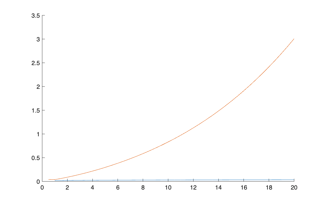
% problem with the forward_rates chart, which does not come out right
% (not saved because wrong) print('G_StrutturaTassi','-djpeg')

function [v] = F_Bootstrap(z)
n = length(z)
z = reshape(z, 1, n)
A = repmat(z, n, 1)
A = tril(A)
A = A + eye(n)
v = A \ ones(n, 1)
end

function [v_int] = F_StructInterYield(t, v, t_int)
y = -log(v) ./ t
y_int = interp1(t, y, t_int)
v_int = exp(-y_int .* t_int)
end

function [forward_prices,forward_rates] = F_forward(t,v)
n = length(t);
forward_prices(1) = v(1);
for k = 2 : n
   forward_prices(:, k) = v(k) / v(k-1)
end

forward_rates(1) = (1 / forward_prices(k)) ^ (1/t(1)) - 1;
for k = 2 : n
    forward_rates(:, k) = (1 / v(k)) ^ (1 / (t(k) - t(k-1))) - 1
end
end

The chart as the submitted code produces it: the continuous spot curve (blue, almost flat at this scale) and the "forward rates" (orange), which climb to 300%.

Spot and forward rates as produced by the submitted code

Task 2 · Mean-variance and mean-MAD frontiers¶

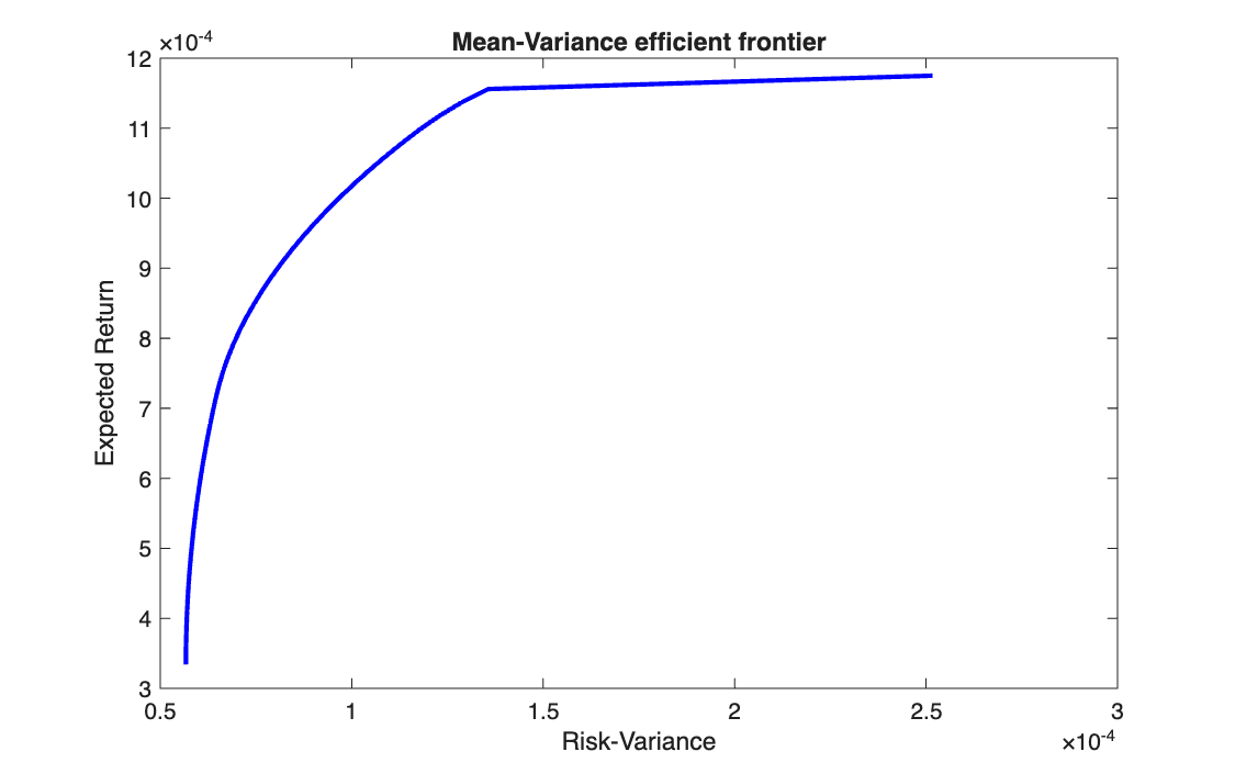
On 12 EURO STOXX 50 stocks and 289 returns, build the mean-variance efficient frontier with 45 target returns, then the mean-MAD frontier.

S_Markowitz.m

clear all, clc

%% 1
A = readtable('EuroStoxx50.xlsx');
%% 2
t = A{:, 1};
P = A{:, 2:end};
P_cut = P(1:290, 1:12);
RR = diff(P_cut) ./ P_cut(1:end-1, :);
mu = mean(RR);
sigma = cov(RR);
[T, n] = size(RR);
%% 3
H = 2 * sigma;
lb = [zeros(n, 1)];
beq = [1];
Aeq = [ones(1, n)];
X_min = quadprog(H,[],[],[],Aeq,beq,lb,[]);
eta_min = mu * X_min
eta_max = max(mu)
eta = linspace(eta_min, eta_max, 45);
%% 4
Aeq_ = [mu; ones(1, n)]
for k = 1 : length(eta)
    beq_ = [eta(k); 1]
    [X,Risk_sigma2(:, k)] = quadprog(H,[],[],[],Aeq_,beq_,lb,[]);
end
%% 5
 save('FrontieraMV.xls','Risk_sigma2')
 plot(Risk_sigma2, eta, 'b', LineWidth=2)
 xlabel('Risk-Variance')
 ylabel('Expected Return')
 title('Mean-Variance efficient frontier')
 print('G_FrontieraMV','-djpeg')
%% 6
% plotting the number of stocks against the target return eta would show
% that as the required return eta(k) grows, the number of stocks
% selected falls (down to a single stock, the one with the highest
% return)

%% 7
dev = RR - repmat(mu, T, 1)
eta_2 = linspace(eta_min, eta_max, 100)
A_1 = [dev, -eye(T),
    -dev, -eye(T)]
f_1 = [zeros(n, 1); ones(T, 1)/ T]
b_1 = [zeros(2*T, 1)]
LB_1 = [zeros(n +T, 1)]

Aeq_1 = [mu, zeros(1, T),
    ones(1, n), zeros(1, T)]
for k = 1 : length(eta_2)
    beq_1 = [eta(k); 1]
    Risk_MAD_(:, k) = linprog(f_1,A_1,b_1,Aeq_1,beq_1,LB_1,[])
end
Risk_MAD = Risk_MAD_(1:n)
figure(2)
plot(Risk_MAD, eta_2)

The mean-variance part runs: the frontier goes from the minimum-variance portfolio (mean return 0.033% per period, variance \(5.7 \times 10^{-5}\), 9 stocks) to the best single stock (0.118%).

Mean-variance efficient frontier from the exam

The mean-MAD part (point 7) stops with an error; see below.

Task 3 · European option: Monte Carlo, binomial tree, Black–Scholes¶

Price a two-year call and put with \(S_0 = 85\), \(K = 90\), \(r = 6\%\), \(\sigma = 40\%\), by Monte Carlo (100,000 draws), on a 24-step binomial tree, and with the Black–Scholes formula.

S_OptionPricing.mF_Montecarlo.mF_Binomiale.m

clear all, clc

%% 1
K = 90;
S_0 = 85;
r = 0.06;
T = 2;
sigma = 0.4;
N = 24;
n = 100000;
[C, P] = F_Montecarlo(S_0, sigma, r, T, K, n)
%% 2
[call_prices,put_prices, put_call_parity] = F_Binomiale(S_0, T, K, r, sigma, N)
% error: the put price does not come out
%% 3
% Black-Scholes formula
d_1 = (log(S_0 ./ K) + (r + (sigma.^2)/2) .* T) / sigma .* sqrt(T)
d_2 = d_1 - sigma .* sqrt(T)
C__ = S_0 * d_1 - K * exp(-r*T) * d_2
P__ = K * exp(-r*T)*(-d_2)- S_0*(-d_1)

function [C, P] = F_Montecarlo(S_0, sigma, r, T, K, n)
z = randn(n, 1);
S_T = S_0 * exp((r - 0.5*sigma^2)*T + sigma*sqrt(T) * z);
C = exp(-r*T) * mean(max(S_T - K,0))
P = exp(-r*T) * mean(max(K - S_T,0))
end

function [call_prices,put_prices, put_call_parity] = F_Binomiale(S_0, T, K, r, sigma, N)
% note: N is the m of the exam text

dt = T / N

% r = log(1 + i)

u = exp(sigma*sqrt(dt))

d = 1 / u

q = (exp(r*dt) - d) / (u - d)

for k = 0 : N

    nodesCall(k+1, N+1) = max(S_0 * u^k *d^(N - k) - K, 0)
    nodesPut(k+1, N+1) = max(K - S_0 * u^k *d^(N - k), 0 )

end

for j = N-1 : -1 :0
    for k = 0 : j
    nodesCall(k+1, j+1) = exp(-r*dt)* (q * nodesCall(k+2, j+2) + (1 - q)*nodesCall(k+1, j+2))
    nodesPut(k+1, j+1) = exp(-r*dt)* (q * nodesPut(k+2, j+2) + (1 - q)*nodesPut(k+1, j+2))
    end
end

call_prices = nodesCall(1,1)
put_prices = nodesPut(1,1)

put_call_parity = call_prices - S_0 + K * exp(-r*T)

	Monte Carlo	Binomial tree, 24 steps	Black–Scholes as submitted	Black–Scholes, correct
Call	20.9285	21.1284	49.2335	21.0519
Put	15.8648	15.9512	49.2335	15.8748

Monte Carlo and the tree agree with the correct closed form; the submitted formula does not.

Errors found on review¶

Task	Where	What is wrong	Effect	Correct result
1	`F_Bootstrap`	`z` is made a row and repeated down the rows, so the matrix has \(A_{ij} = z_j\) instead of \(z_i\): each equation uses the other maturities' rates	the curve is too low	20-year spot 4.22% (annual), not 3.53%
1	`F_forward`	the first forward rate uses `forward_prices(k)`, the last one, instead of `forward_prices(1)`; the others use the spot price `v(k)` instead of the forward price	"forward rates" rise to 300%	forward rates between 2.6% and 5.0%
1	`F_StructInterYield`	the 6-month point is before the first maturity (1 year) and is not extrapolated	the curves start at 1 year	minor
2	point 7	the loop runs over the 100 targets of `eta_2` but reads `eta(k)`, which has 45	stops at \(k = 46\) with "Index exceeds the number of array elements"	—
2	point 7	`linprog` is asked only for the solution vector, so `Risk_MAD_` stores weights and auxiliary variables, not the MAD; `Risk_MAD_(1:n)` then takes the first \(n\) entries of one column	even without the index error, the plotted "risk" would not be the MAD	the MAD is the second output of `linprog`
3	Black–Scholes	`d_1` is divided by `sigma` and then multiplied by `sqrt(T)` instead of divided by `sigma*sqrt(T)`; the prices use `d_1` and `d_2` directly instead of \(N(d_1)\) and \(N(d_2)\)	call = put = 49.23	call 21.0519, put 15.8748

The comment in S_OptionPricing.m says the binomial tree does not give the put price. When the code is run, it does: 15.9512, equal to the put-call parity check.

The correct formulas for all three tasks are on the course pages: bootstrapping, spot and forward curve, mean-MAD frontier, binomial tree.