Simulating geometric Brownian motion
Problem
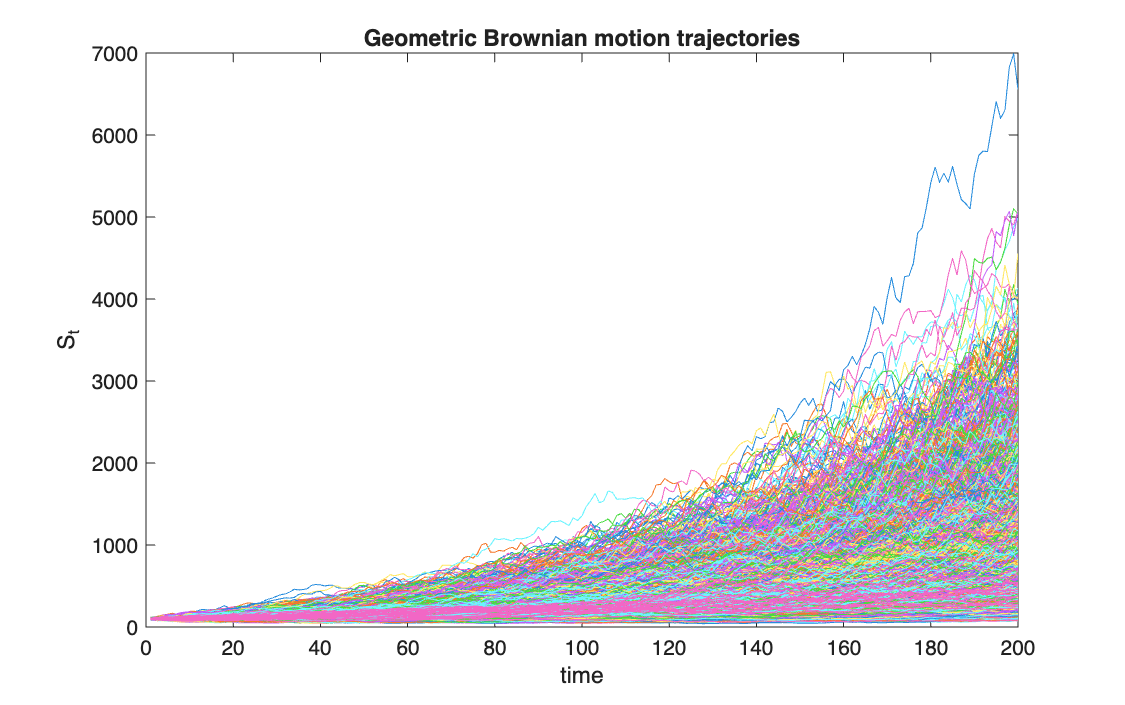
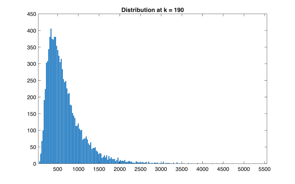
Simulate 10,000 price paths following a geometric Brownian motion, the model behind Black–Scholes, over 200 steps, and study the distribution of the price across paths over time.
Method
The logarithm of the price follows a Brownian motion, so the price itself is:
\[
S_{t} = S_0 \exp\!\Big(\big(\mu - \tfrac12\sigma^2\big)t + \sigma W_t\Big)
\]
simulated by cumulating the increments of \(\ln S\), \((\mu - \tfrac12\sigma^2)\Delta t + \sigma\sqrt{\Delta t}\,Z\). Then \(S_t\) is log-normal, with \(\mathbb{E}[S_t] = S_0 e^{\mu t}\) and median \(S_0 e^{(\mu - \sigma^2/2)t}\). Here \(S_0 = 100\), \(\mu = 0.2\), \(\sigma = 0.2\), \(\Delta t = 0.05\).
Code
clear all, clc

%% 1

n = 10000;
m = 200;
mu = 0.2;
sigma = 0.2;
Dt = 0.05;
S_0 = 100;

Z    = randn(n, m);
dX   = (mu - 0.5*sigma^2)*Dt + sigma*sqrt(Dt)*Z;   % increments of ln(S)
S_tk = S_0 * exp(cumsum(dX, 2));                   % S_tk = S_0 * e^{sum of the increments}

%% 2

save('GeoBM.txt', 'S_tk', '-ascii', '-tabs')

%% 3

figure(1)
plot(S_tk')
xlabel('time'); ylabel('S_t'); title('Geometric Brownian motion trajectories')

%% 4

for k = 10:20:190
    figure
    F_Empirical_pdf(S_tk(:, k), 200);
    title(['Distribution at k = ', num2str(k)])
    print('-djpeg', ['GeoBM', num2str(k)])
end
import numpy as np
import matplotlib.pyplot as plt
from F_Empirical_pdf import F_Empirical_pdf

# %% 1
n = 10000
m = 200
mu = 0.2
sigma = 0.2
Dt = 0.05
S_0 = 100

Z = np.random.randn(n, m)
dX = (mu - 0.5 * sigma**2) * Dt + sigma * np.sqrt(Dt) * Z   # increments of ln(S)
S_tk = S_0 * np.exp(np.cumsum(dX, axis=1))                  # S_tk = S_0 * e^(sum of the increments)

# %% 2
np.savetxt('GeoBM.txt', S_tk, delimiter='\t')

# %% 3
plt.figure(1)
plt.plot(S_tk.T)
plt.xlabel('time'); plt.ylabel('S_t'); plt.title('Geometric Brownian motion trajectories')

# %% 4
for k in range(10, 191, 20):
    plt.figure()
    F_Empirical_pdf(S_tk[:, k-1], 200)
    plt.title('Distribution at k = ' + str(k))
    plt.savefig('GeoBM' + str(k) + '.jpg')

plt.show()
In MATLAB, the helper F_Empirical_pdf is the one shown in Part II.
Results
| Step \(k\) | Time \(t\) | Mean (theory) | Median (theory) | Skewness |
|---|---|---|---|---|
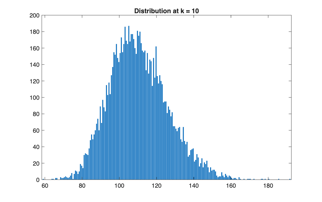
| 10 | 0.5 | 110.5 (110.5) | 109.3 (109.4) | 0.42 |
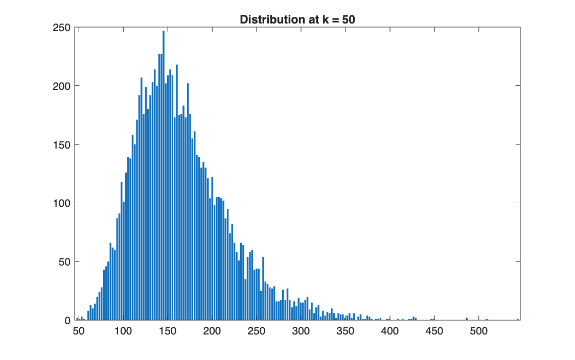
| 50 | 2.5 | 165.0 (164.9) | 156.1 (156.8) | 1.04 |
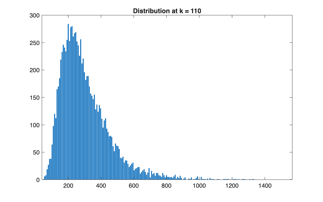
| 110 | 5.5 | 302.5 (300.4) | 269.1 (269.1) | 1.66 |
| 190 | 9.5 | 672.4 (668.6) | 555.1 (552.9) | 2.21 |
Takeaways
- Prices stay positive and their distribution becomes more and more right-skewed: a few paths go very high (close to 7,000 from 100), most stay much lower.
- The mean grows at \(\mu\), but the median grows only at \(\mu - \sigma^2/2\): the typical path is below the average one, and the gap widens over time.
- This is the same log-normal of Part II, now evolving in time; it is what the Monte Carlo pricers on the next pages simulate.