Present value of an annuity
Problem
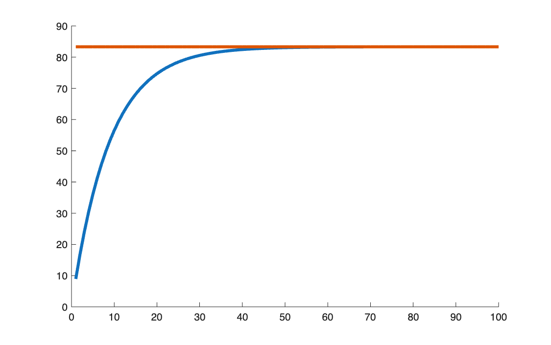
Compute the present value of an annuity paying 10 a year for 17 years at 12%, first with a loop and then with the closed form. Then plot how the value changes with the number of payments, up to 100.
Method
\[
V_0 = \sum_{k=1}^{n} R\, v^k = R\, v\, \frac{1 - v^n}{1 - v}, \qquad v = \frac{1}{1+i}
\]
As \(n \to \infty\) the annuity becomes a perpetuity, worth \(R / i\).
Code
clear all, clc

%% 1

i = 12/100;
R = 10;
n = 17;
v = 1 / (1 + i);

V_0 = 0;

for k = 1 : n

    V_0 = V_0 + R * v^k;

end

V_0

% check
V_0_check = R * v * ((1 - v^n) / (1 - v))

%% 2

n_graph = 1:100;

V_0_graph = R * v * ((1 - v.^n_graph) / (1 - v));

asymptote = R / i

figure(1)
hold on
plot(n_graph, V_0_graph, linewidth=3)
plot(n_graph, asymptote*ones(1, 100), linewidth=3)
hold off
import numpy as np                 # vectors and maths (the "MATLAB" part of Python)
import matplotlib.pyplot as plt    # charts (figure, plot, hold on...)

# %% 1

i = 12/100
R = 10
n = 17
v = 1 / (1 + i)

V_0 = 0

for k in range(1, n + 1):          # MATLAB: for k = 1 : n   (the end of range is excluded, hence n + 1)

    V_0 = V_0 + R * v**k           # ** is the power, MATLAB's ^

print("V_0 =", V_0)                # no ; to suppress output in Python: print what you want to see

# check
V_0_check = R * v * ((1 - v**n) / (1 - v))
print("V_0_check =", V_0_check)

# %% 2

n_graph = np.arange(1, 101)        # MATLAB: 1:100   (again, the end is excluded)

V_0_graph = R * v * ((1 - v**n_graph) / (1 - v))   # on a numpy vector, ** works element by element, like .^

asymptote = R / i
print("asymptote =", asymptote)

plt.figure(1)                      # hold on is the default in matplotlib
plt.plot(n_graph, V_0_graph, linewidth=3)
plt.plot(n_graph, asymptote * np.ones(100), linewidth=3)
plt.show()
Results
Loop and closed form agree: \(V_0 = 71.1963\). The perpetuity value is \(R/i = 83.33\).
Takeaways
- The closed form is a geometric series; the loop is a way to check it.
- Adding payments adds less and less value: at 12%, the 17-year annuity is already worth 85% of a perpetuity.