Portfolio value under scenarios and Monte Carlo VaR
Problem
A portfolio holds five stocks, with current prices \(P_0\) and share quantities \(q\). Given a matrix of three return scenarios, compute the portfolio value and return in each one. Then replace the three scenarios with 100 simulated ones and estimate the 95% Value at Risk.
Method
The portfolio value is the price vector times the quantities, today and in each scenario \(s\):
\[
V_0 = P_0\, q^\top, \qquad V_s = \big(P_0 \circ (1 + R_s)\big)\, q^\top, \qquad R^{p}_s = \frac{V_s}{V_0} - 1
\]
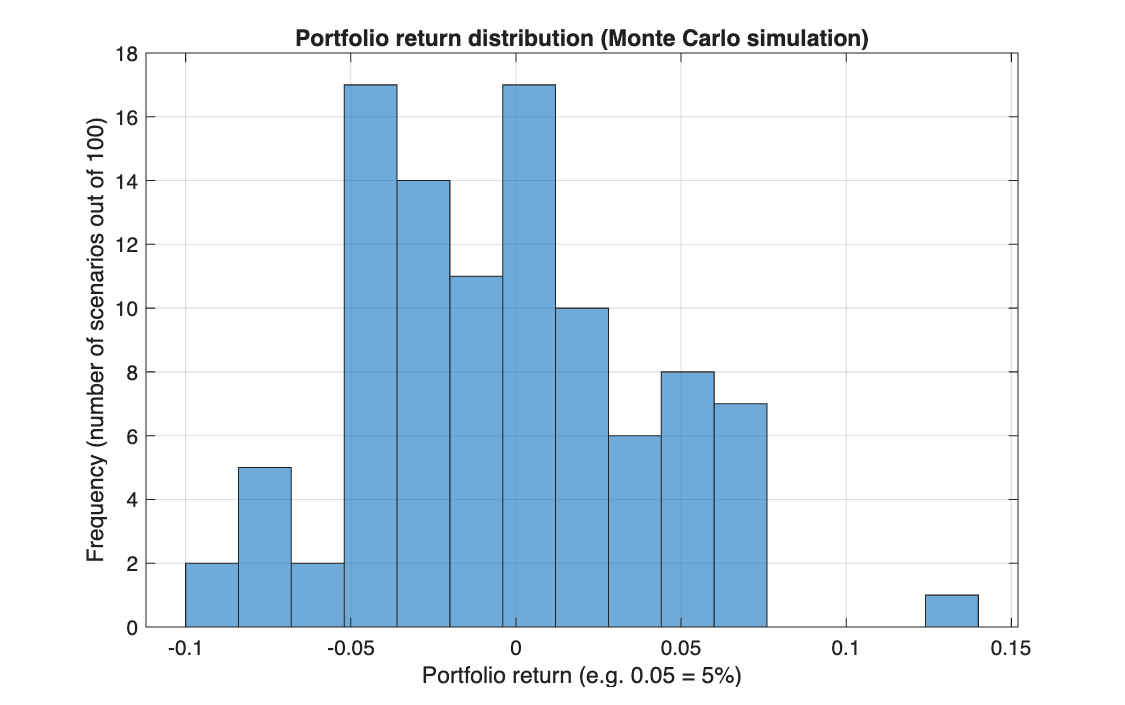
For the simulation, each stock's return is drawn from \(\mathcal{N}(0,\, 0.1^2)\). The 95% VaR is the 5th percentile of the 100 simulated portfolio returns.
Code
clear all, clc

% Point 1

    % input of daily return matrix R
    R = [ 0.03,  0.05,  0.04,  0.02,  0.05;
          0.05,  0.06,  0.05,  0.03,  0.08;
         -0.04, -0.02,  0.01, -0.01, -0.10];

    [n, m] = size(R);                 % n (rows) are the scenarios, m (columns) are the stocks

    P_0 = [10, 20, 15, 20, 25];       % current price vector (at time 0)

    P = repmat(P_0, n, 1) .* (1 + R); % calculation of asset price simulation matrix
    % new price = current price * (1 + rate of return)
    % repmat replicates the row vector so it can be multiplied by each scenario in R

    q = [1000, 800, 1100, 700, 500];  % input of the stock share vector (number of shares held for each stock)

    V_q = P * q';                     % value of the portfolio for each scenario

    V_0 = P_0 * q';                   % current portfolio value

    R_q = (V_q / V_0) - 1;            % portfolio return for each scenario
    % (final value / initial value) - 1: one return per scenario (the three rows of R)


% Point 2 - Monte carlo simulation

    % given the previously introduced:
    %    m      number of stocks
    %    q      stock shares
    %    P_0    current price vector
    %    V_0    current portfolio value

    % Instead of three given scenarios, generate 100 random ones and see
    % how the portfolio behaves across them. The last three steps are the
    % same as in Point 1.

    n_MC = 100;                       % n_MC are the scenarios of the Monte Carlo simulation

    R_MC = randn(n_MC, m) / 10;       % simulation of a multivariate normal rv
    % 100 x 5 matrix of normal returns; dividing by 10 gives a 10% volatility

    P_MC = repmat(P_0, n_MC, 1) .* (1 + R_MC); % calculation of asset price simulation matrix

    V_MC_q = P_MC * q';               % value of the portfolio for each scenario

    R_MC_q = (V_MC_q / V_0) - 1;      % portfolio return for each scenario


% extra: histogram of the simulated returns

    figure;
    histogram(R_MC_q, 15);            % 15 bins

    title('Portfolio return distribution (Monte Carlo simulation)');
    xlabel('Portfolio return (e.g. 0.05 = 5%)');
    ylabel('Frequency (number of scenarios out of 100)');
    grid on;


% extra: 95% Value at Risk

    % "With 95% confidence, the portfolio will not lose more than X"

    % 1. confidence level
    livello_confidenza = 95;
    percentile_var = 100 - livello_confidenza; % the 5% threshold

    % 2. VaR as a return, from the percentile of the simulated returns
    VaR_95_perc = prctile(R_MC_q, percentile_var);

    % 3. print the result as a percentage
    fprintf('95%% VaR of the portfolio: %.2f%%\n', VaR_95_perc * 100);

    % 4. the same loss in currency
    VaR_95_valore = V_0 * VaR_95_perc;
    fprintf('Estimated maximum loss at 95%%: %.2f EUR\n', VaR_95_valore);
import numpy as np
import matplotlib.pyplot as plt

# %% Point 1

# input of daily return matrix R
R = np.array([[ 0.03,  0.05,  0.04,  0.02,  0.05],
              [ 0.05,  0.06,  0.05,  0.03,  0.08],
              [-0.04, -0.02,  0.01, -0.01, -0.10]])

n, m = R.shape                          # n (rows) are the scenarios, m (columns) are the stocks

P_0 = np.array([10, 20, 15, 20, 25])    # current price vector (at time 0)

P = np.tile(P_0, (n, 1)) * (1 + R)      # MATLAB: repmat(P_0, n, 1) .* (1 + R)   (* is element by element)

q = np.array([1000, 800, 1100, 700, 500])   # number of shares held for each stock

V_q = P @ q                             # value of the portfolio for each scenario   (@ is the matrix product, MATLAB's *)

V_0 = P_0 @ q                           # current portfolio value

R_q = (V_q / V_0) - 1                   # portfolio return for each scenario

# %% Point 2 - Monte Carlo simulation

n_MC = 100                              # scenarios of the Monte Carlo simulation

R_MC = np.random.randn(n_MC, m) / 10    # 100 x 5 matrix of normal returns, 10% volatility

P_MC = np.tile(P_0, (n_MC, 1)) * (1 + R_MC)

V_MC_q = P_MC @ q

R_MC_q = (V_MC_q / V_0) - 1

# %% extra: histogram of the simulated returns

plt.figure()
plt.hist(R_MC_q, 15)                    # 15 bins
plt.title('Portfolio return distribution (Monte Carlo simulation)')
plt.xlabel('Portfolio return (e.g. 0.05 = 5%)')
plt.ylabel('Frequency (number of scenarios out of 100)')
plt.grid(True)

# %% extra: 95% Value at Risk

livello_confidenza = 95
percentile_var = 100 - livello_confidenza

VaR_95_perc = np.percentile(R_MC_q, percentile_var)     # MATLAB: prctile
print(f"95% VaR of the portfolio: {VaR_95_perc * 100:.2f}%")   # f"...{x:.2f}..." is MATLAB's fprintf('%.2f', x)

VaR_95_valore = V_0 * VaR_95_perc
print(f"Estimated maximum loss at 95%: {VaR_95_valore:.2f} EUR")

plt.show()
Results
Today's value is \(V_0 = 69{,}000\). In the three given scenarios:
| Scenario | Portfolio value | Return |
|---|---|---|
| 1 | 71,665 | +3.86% |
| 2 | 72,705 | +5.37% |
| 3 | 67,055 | −2.82% |
On one simulated run (random seed fixed at 0 when generating this page), the 95% VaR is −7.10%, a loss of 4,901.54 EUR.
Takeaways
- The portfolio return is the change in total value, so each stock weighs by price times quantity, not by number of shares.
- The matrix form (\(P\,q^\top\)) values every scenario in one line: no loop over scenarios.
- A VaR estimated from 100 scenarios is noisy: a different seed gives a visibly different number. More scenarios, or a closed form, give a stable one.