Simulating Brownian motion
Problem
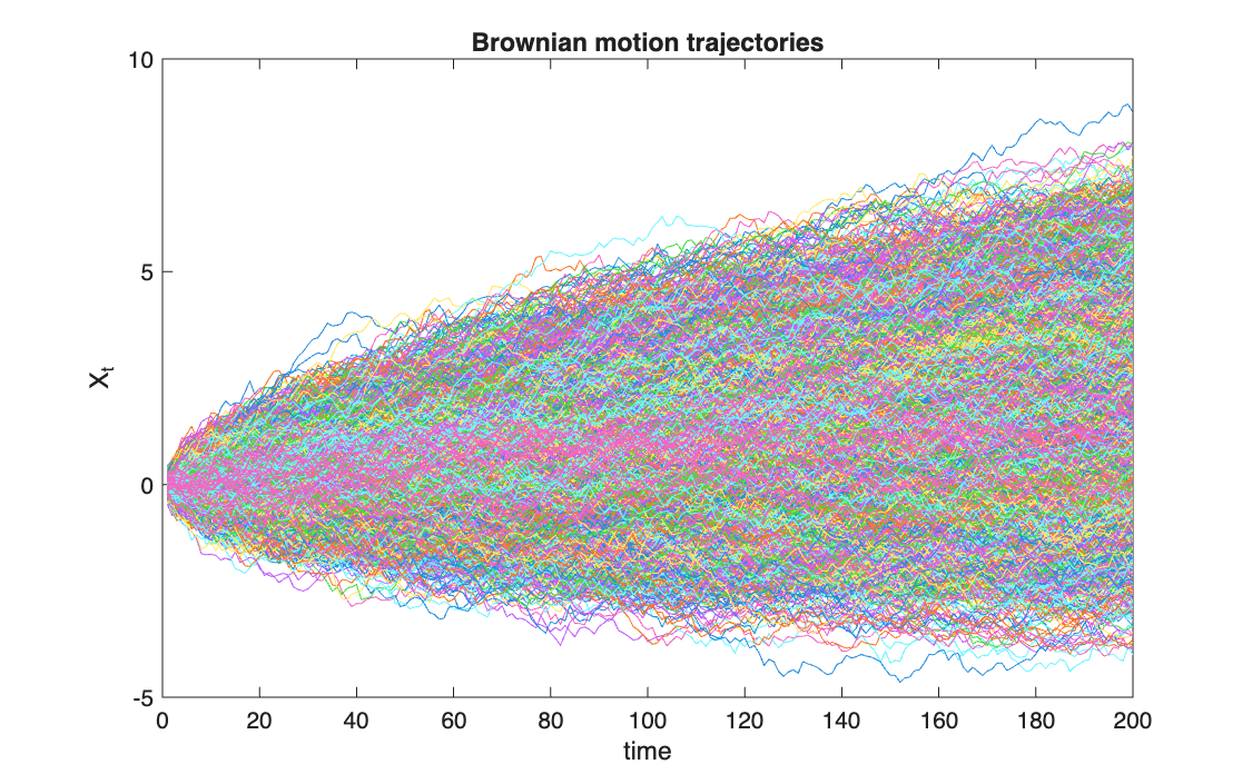
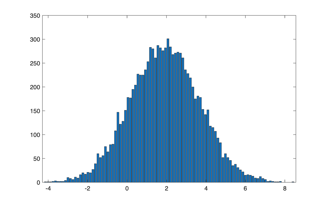
Simulate 10,000 paths of a Brownian motion with drift, over 200 steps, and study how the distribution of the process across paths changes over time.
Method
With drift \(\mu\) and diffusion \(\sigma\), each step adds a normal increment:
\[
X_{k} = X_{k-1} + \mu\,\Delta t + \sigma\sqrt{\Delta t}\;Z_k, \qquad Z_k \sim \mathcal{N}(0,1)
\]
so that \(X_t \sim \mathcal{N}(X_0 + \mu t,\ \sigma^2 t)\). All increments are generated at once as an
\(n \times m\) matrix, and cumsum along each row builds the paths. Here \(\mu = 0.1\),
\(\sigma = 0.4\), \(\Delta t = 0.1\), \(X_0 = 0\).
Code
clear all, clc

%% 1

n     = 10000;   % number of trajectories
m     = 200;     % number of time steps
mu    = 0.1;     % drift
sigma = 0.4;     % volatility (diffusion)
Dt    = 0.1;     % time step

X = F_BrownMot(mu, sigma, m, Dt, n);   % x_0 omitted -> default 0 (nargin)

%% 2

save('BrownMot.txt', 'X', '-ascii', '-tabs')

%% Point 3

figure(1)
plot(X')
xlabel('time');
ylabel('X_t');
title('Brownian motion trajectories')

%% Point 4

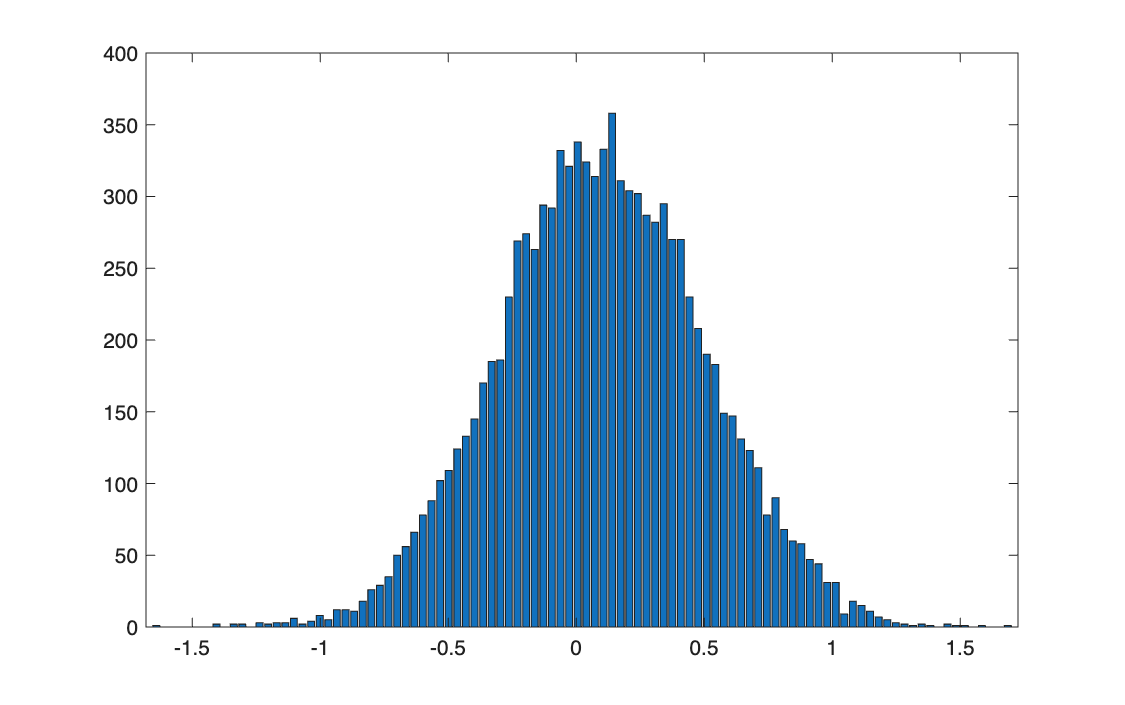
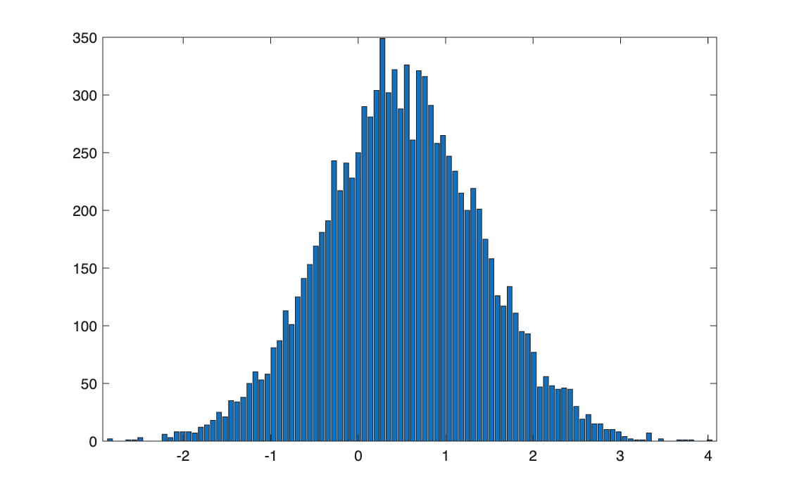
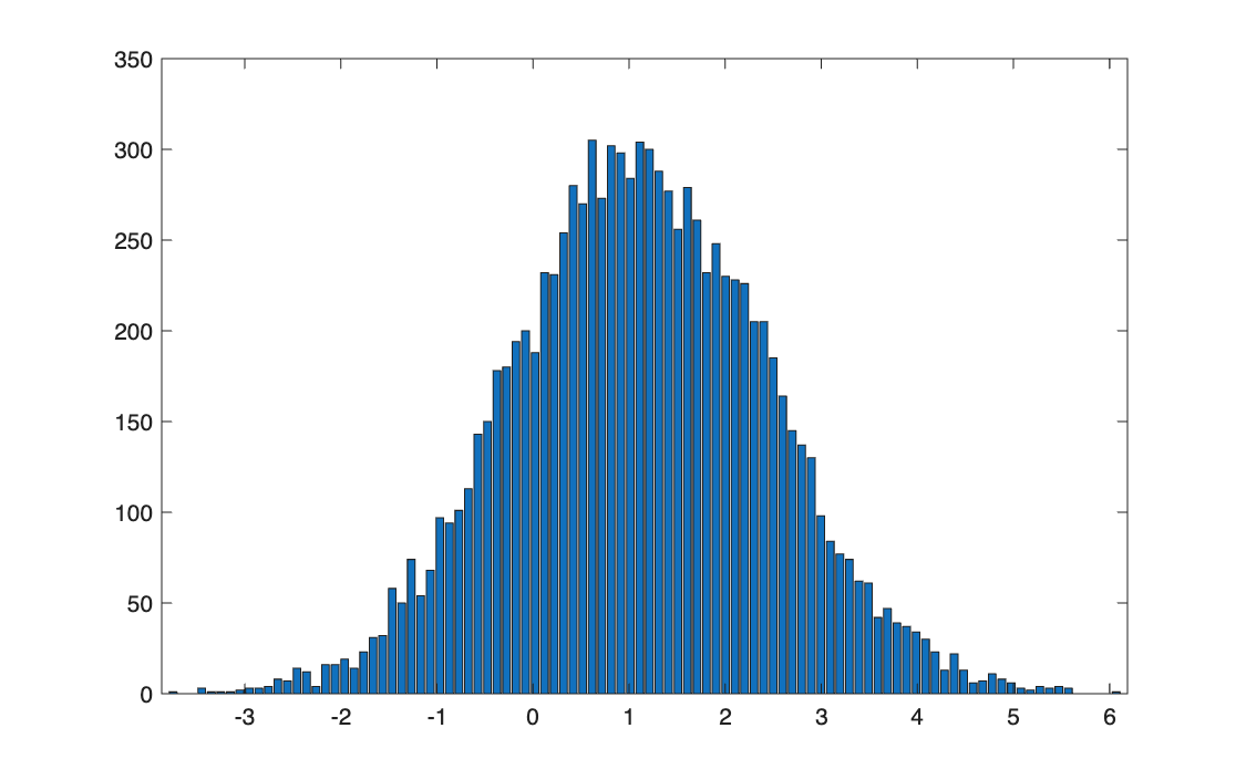
for k = 10:20:190
    figure
    F_Empirical_pdf(X(:, k), 100);
    print('-djpeg',['BrownMot',num2str(k)])
end


function [X] = F_BrownMot(mu, sigma, m, Dt, n, x_0)
% Simulates n trajectories of a Brownian motion with drift mu and diffusion
% sigma, over m steps of length Dt. Formula: dX_k = mu*Dt + sigma*sqrt(Dt)*Z (5.8, p. 190)

    if nargin == 5
        x_0 = 0;                       % default initial value (textbook, p. 190)
    end

    Z  = randn(n, m);                  % N(0,1) shocks: n simulations x m steps (point 1)
    dX = mu*Dt + sigma*sqrt(Dt)*Z;     % increments (point 2)
    X = x_0 + cumsum(dX, 2);                % X_k = X_0 + sum of the increments (point 3, cumsum)

end
import numpy as np
import matplotlib.pyplot as plt
from F_Empirical_pdf import F_Empirical_pdf


# %% function F_BrownMot

def F_BrownMot(mu, sigma, m, Dt, n, x_0=0):     # x_0=0: default value, MATLAB uses nargin for this
    # n trajectories of a Brownian motion with drift mu and diffusion sigma,
    # over m steps of length Dt:  dX_k = mu*Dt + sigma*sqrt(Dt)*Z

    Z = np.random.randn(n, m)           # N(0,1) shocks: n simulations x m steps
    dX = mu * Dt + sigma * np.sqrt(Dt) * Z      # increments
    X = x_0 + np.cumsum(dX, axis=1)     # MATLAB: cumsum(dX, 2)   (axis=1: along each row)
    return X


# %% 1
n = 10000       # number of trajectories
m = 200         # number of time steps
mu = 0.1        # drift
sigma = 0.4     # volatility (diffusion)
Dt = 0.1        # time step

X = F_BrownMot(mu, sigma, m, Dt, n)     # x_0 omitted -> default 0

# %% 2
np.savetxt('BrownMot.txt', X, delimiter='\t')  # MATLAB: save('BrownMot.txt', 'X', '-ascii', '-tabs')

# %% Point 3
plt.figure(1)
plt.plot(X.T)                           # MATLAB: plot(X')   (.T is the transpose)
plt.xlabel('time')
plt.ylabel('X_t')
plt.title('Brownian motion trajectories')

# %% Point 4
for k in range(10, 191, 20):            # MATLAB: for k = 10:20:190
    plt.figure()
    F_Empirical_pdf(X[:, k-1], 100)     # MATLAB: X(:, k)   (column k is k-1 in Python)
    plt.savefig('BrownMot' + str(k) + '.jpg')   # MATLAB: print('-djpeg', ['BrownMot', num2str(k)])

plt.show()
Results
| Step \(k\) | Time \(t\) | Mean (theory) | Standard deviation (theory) |
|---|---|---|---|
| 10 | 1 | 0.099 (0.100) | 0.399 (0.400) |
| 50 | 5 | 0.501 (0.500) | 0.900 (0.894) |
| 110 | 11 | 1.115 (1.100) | 1.332 (1.327) |
| 190 | 19 | 1.912 (1.900) | 1.748 (1.744) |
Takeaways
- The distribution stays normal at every time; it drifts at speed \(\mu\) and widens as \(\sqrt{t}\), not as \(t\).
- The drift is small compared with the noise: after 19 time units the mean is 1.9 but the standard deviation is 1.7, so many paths still end below zero.
- Generating the whole increment matrix and cumulating it is the vectorised form of the loop over time steps.