How correlation shapes the frontier¶

Course exercise 132 · Part II

Problem¶

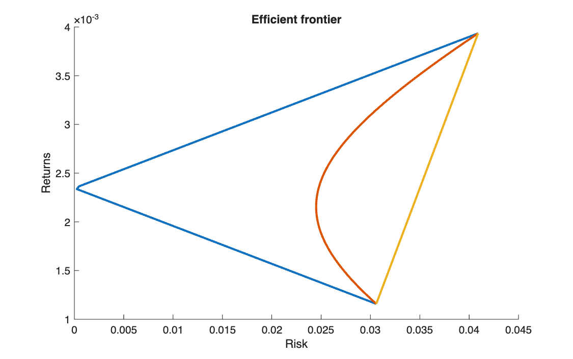
Take two stocks from the EURO STOXX 50 data and keep their own expected returns and volatilities, but impose three correlations between them: −1, 0 and +1. Plot the three resulting frontiers.

Method¶

With two assets, the portfolio variance for weights \(x_1 + x_2 = 1\) is

\[ \sigma_p^2 = x_1^2 \sigma_1^2 + x_2^2 \sigma_2^2 + 2\,x_1 x_2\,\rho\,\sigma_1 \sigma_2 \]

The covariance matrix is rebuilt for each \(\rho\) and the frontier is traced with quadprog over target returns between the two stocks' returns; the risk axis is the volatility \(\sigma_p\).

Code¶

MATLABPython

S_exercise_132.m

clear all, clc

%% 1

A = readtable("weekly_EUROSTOXX50_price_time.txt");
times = A{:, 1};
P = A{:, [6 7]};

%% 2

Ret = diff(P) ./ P(1:end-1, :);
[n_valori, n_asset] = size(Ret);

%% 3

mu  = mean(Ret);
vol = std(Ret); % sigma = standard deviation = volatility  (sigma^2 = variance)

eta_min = min(mu);
eta_max = max(mu);
eta = linspace(eta_min, eta_max, 100);

rho = [-1 0 1];

Risk_vol = NaN(length(rho), 100);
Aeq_ = [mu; ones(1, n_asset)];
lb   = zeros(n_asset, 1);

%% 4

for j = 1:length(rho)

    Sigma = [vol(1)^2,                rho(j)*vol(1)*vol(2);
             rho(j)*vol(1)*vol(2),    vol(2)^2]; % Sigma = covariance matrix

    H = 2 * Sigma;

    for k = 1:length(eta)
        beq_ = [eta(k); 1];
        [x, Risk_var] = quadprog(H, [], [], [], Aeq_, beq_, lb, []); % Risk_var = portfolio variance (sigma^2)
        Risk_vol(j, k) = sqrt(Risk_var);
    end

end

%% 5

figure(1)
hold on
for k = 1:length(rho)
    plot(Risk_vol(k, :), eta, LineWidth=2)
end
xlabel('Risk')
ylabel('Returns')
title('Efficient frontier')

S_exercise_132.py

import numpy as np
import matplotlib.pyplot as plt
from scipy.optimize import minimize

# %% 1
A = np.loadtxt('weekly_EUROSTOXX50_price_time.txt')
times = A[:, 0]
P = A[:, [5, 6]]                        # MATLAB: A{:, [6 7]}   (columns 6 and 7 are 5 and 6 in Python)

# %% 2
Ret = np.diff(P, axis=0) / P[:-1, :]
n_valori, n_asset = Ret.shape

# %% 3
mu = np.mean(Ret, axis=0)
vol = np.std(Ret, axis=0, ddof=1)       # MATLAB: std(Ret)   (ddof=1 divides by N-1, as MATLAB does)

eta_min = np.min(mu)
eta_max = np.max(mu)
eta = np.linspace(eta_min, eta_max, 100)

rho = [-1, 0, 1]

Risk_vol = np.zeros((len(rho), 100))
lb = [(0, None)] * n_asset
budget = {'type': 'eq', 'fun': lambda x: np.sum(x) - 1}

# %% 4
for j in range(len(rho)):

    Sigma = np.array([[vol[0]**2,                   rho[j] * vol[0] * vol[1]],
                      [rho[j] * vol[0] * vol[1],    vol[1]**2]])     # covariance matrix
    H = 2 * Sigma

    for k in range(len(eta)):
        target = {'type': 'eq', 'fun': lambda x: mu @ x - eta[k]}
        res = minimize(lambda x: 0.5 * x @ H @ x, np.array([0.5, 0.5]), method='SLSQP',
                       bounds=lb, constraints=[budget, target], options={'ftol': 1e-14})
        Risk_var = res.fun              # portfolio variance
        Risk_vol[j, k] = np.sqrt(max(Risk_var, 0))   # volatility (max(...,0) avoids a tiny negative rounding)

# %% 5
plt.figure(1)
for k in range(len(rho)):
    plt.plot(Risk_vol[k, :], eta, linewidth=2)
plt.xlabel('Risk')
plt.ylabel('Returns')
plt.title('Efficient frontier')
plt.show()

Results¶

The two stocks have weekly expected returns of 0.116% and 0.394% and volatilities of 3.06% and 4.09%.

Correlation	Lowest volatility reachable
\(\rho = -1\)	0.03% (practically zero)
\(\rho = 0\)	2.45%
\(\rho = +1\)	3.06% (the less volatile stock alone)

Frontiers of two assets for correlation −1 (blue), 0 (orange) and +1 (yellow)

Takeaways¶

With \(\rho = +1\) there is no diversification: the frontier is a straight line between the two stocks.
With \(\rho = -1\) the two stocks hedge each other perfectly, and a riskless combination exists.
Every real case lies in between: the lower the correlation, the more the curve bends to the left, and the more risk diversification removes.