Simulating random variables
Problem
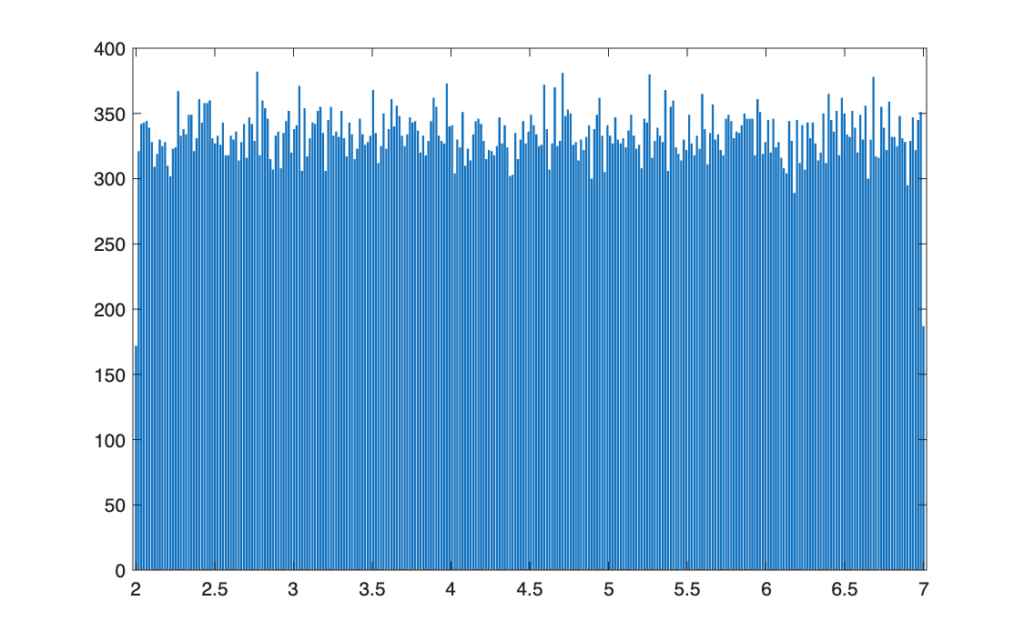
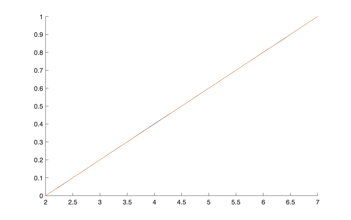
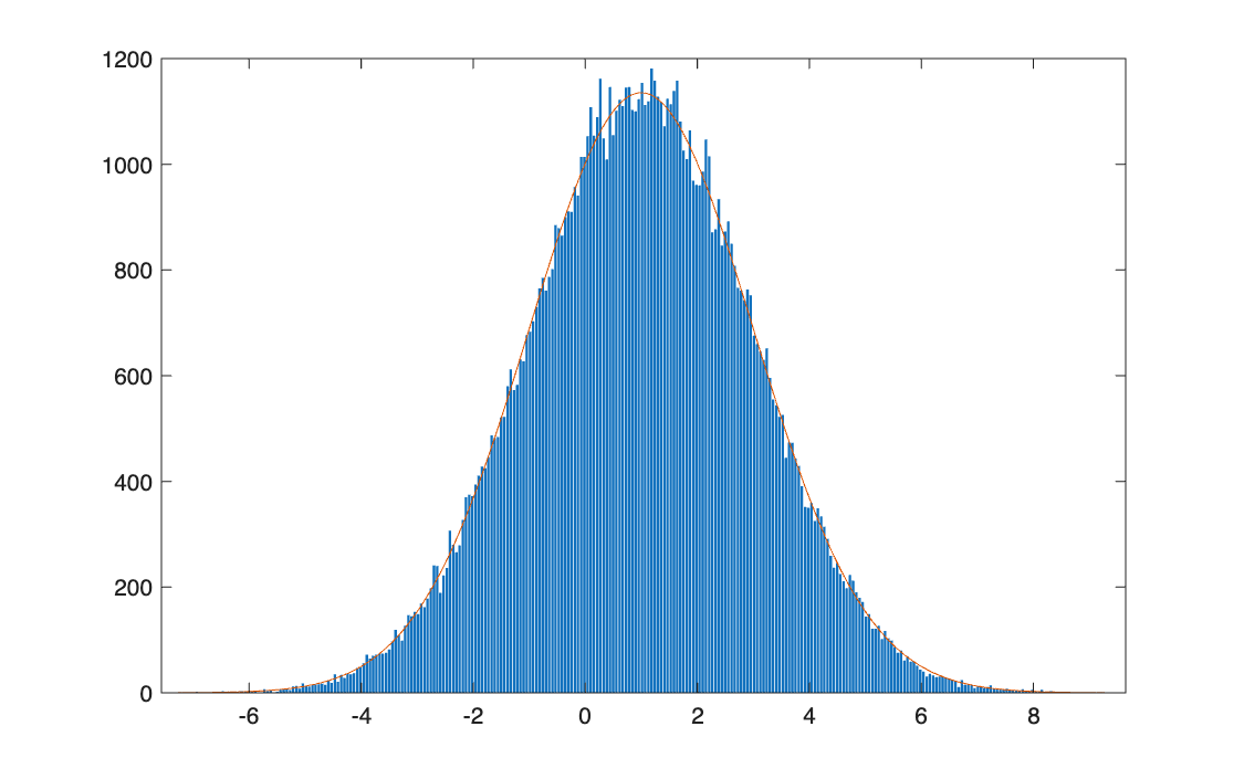
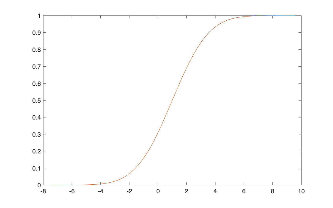
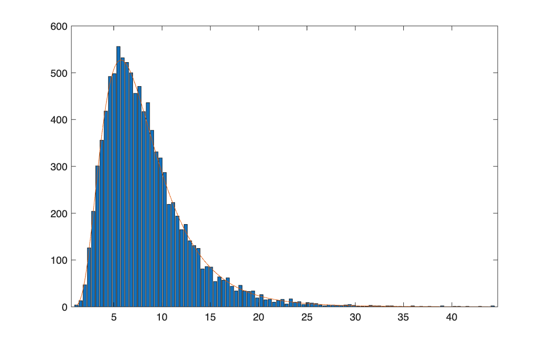
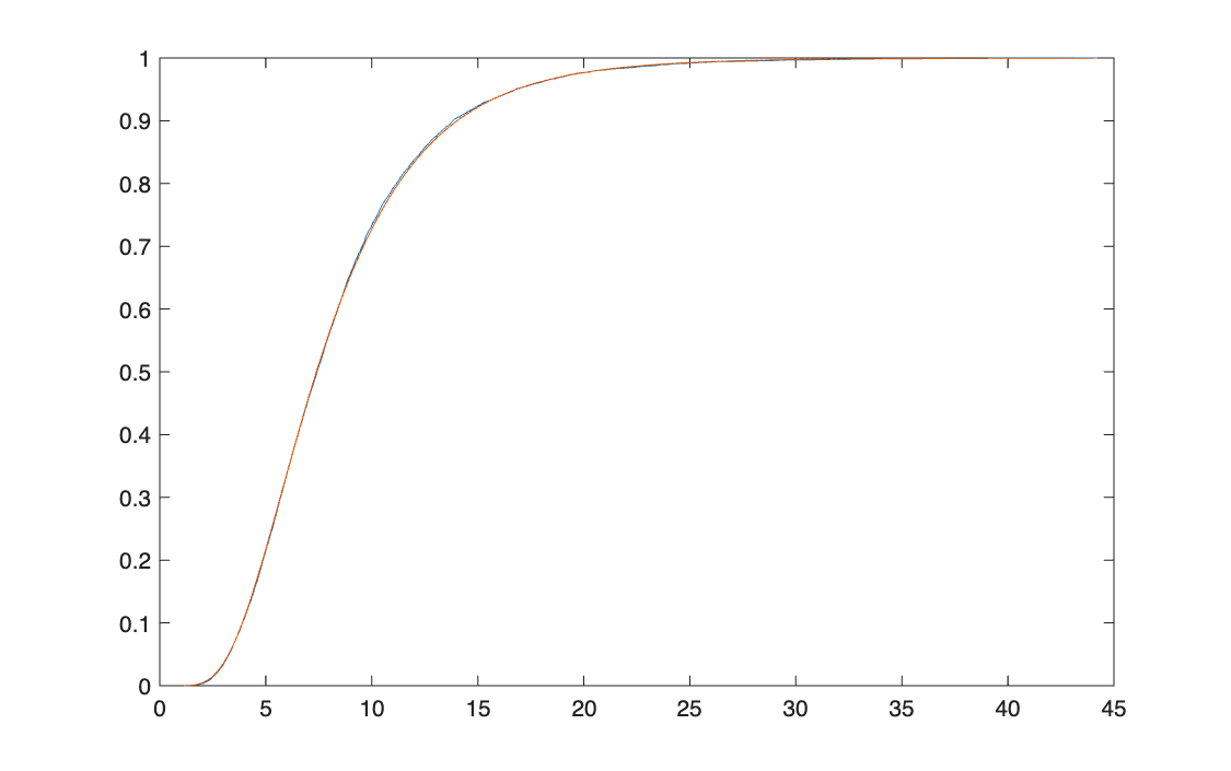
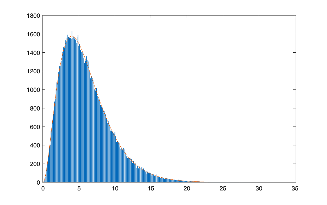
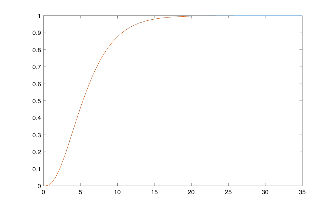
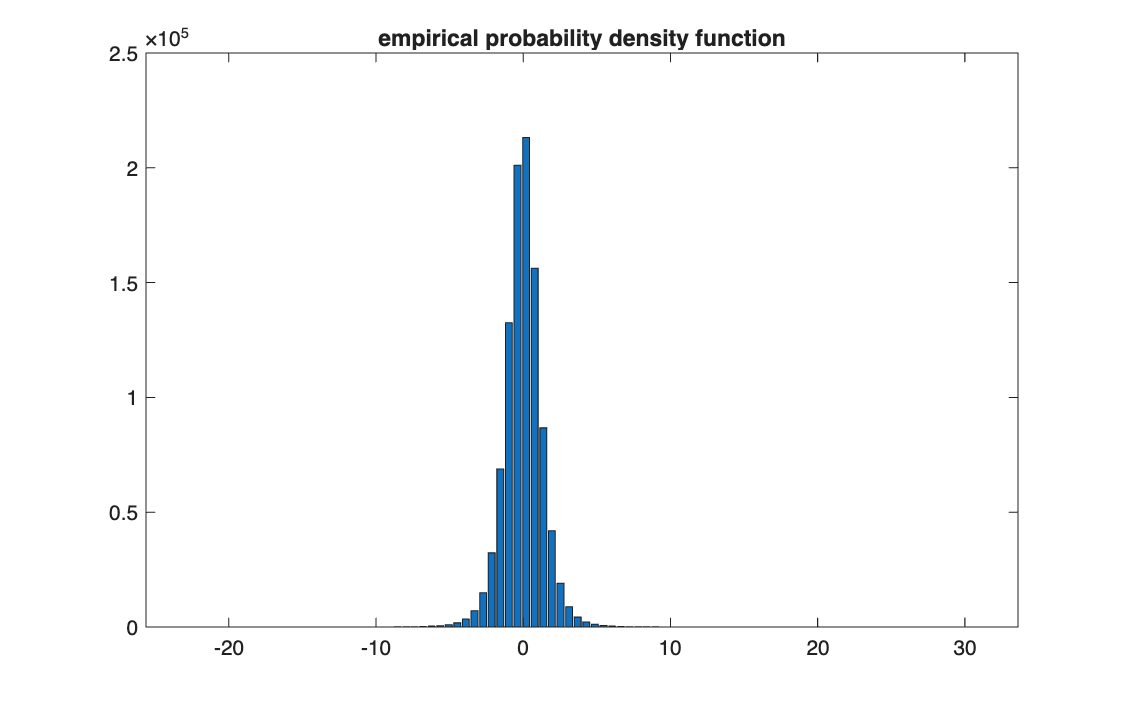
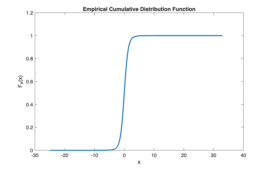
Generate large samples from five distributions, each built from uniform or standard normal draws: uniform, normal, log-normal, chi-square and Student's t. For each, plot the empirical density and CDF against the theoretical ones and compare the sample moments with their theoretical values.
Method
Every distribution is obtained by transforming simple draws, \(Z \sim U[0,1]\) or \(Z \sim \mathcal{N}(0,1)\):
| Distribution | Construction | Exercise |
|---|---|---|
| Uniform \(U[a,b]\) | \(a + (b - a)\,Z\), with \(Z \sim U[0,1]\) | 103 |
| Normal \(\mathcal{N}(\mu, \sigma^2)\) | \(\mu + \sigma Z\) | 107 |
| Log-normal | \(e^{\mu + \sigma Z}\) | 108 |
| Chi-square, \(\nu\) d.o.f. | \(\sum_{j=1}^{\nu} Z_j^2\) | 109 |
| Student's t, \(\nu\) d.o.f. | \(Z_0 \,/\, \sqrt{\tfrac{1}{\nu}\sum_{j=1}^{\nu} Z_j^2}\) | 110 |
To overlay a theoretical density on a histogram of counts, the density is scaled by \(n \times\) bin width.
Code
clear all, clc

%% 1

n = 100000;
a = 2;
b = 7;
x = a + (b - a) * rand(n, 1);
x_plot = linspace(a, b, 1000);   % grid for the theoretical curves

%% 2

nbins = 300;
figure(1)
F_Empirical_pdf(x, nbins)
hold on
plot(x_plot, pdf('Uniform', x_plot, a, b))

%% 3

p = ones(n, 1)/n;
figure(2)
hold on
F_Empirical_cdf(x, p)
plot(x_plot, cdf('Uniform', x_plot, a, b))

%% 4

[E_x, Var_x, Sk_x, Ku_x] = F_SynteticIndices(x)
E_x_   = a + (b - a)/2
Var_x_ = (b - a)^2 / 12
Sk_x_  = 0
Ku_x_  = 9/5
clear all, clc

%% 1

n     = 100000;
mu    = 1;
sigma = 2;
x     = mu + sigma * randn(n, 1);
x_plot = linspace(min(x), max(x), 1000);

%% 2

nbins = 300;
bin_width = (max(x) - min(x)) / nbins;
figure(1)
F_Empirical_pdf(x, nbins)
hold on
plot(x_plot, pdf('Normal', x_plot, mu, sigma) * n * bin_width)
hold off

%% 3

p = ones(n, 1)/n;
figure(2)
F_Empirical_cdf(x, p)
hold on
plot(x_plot, cdf('Normal', x_plot, mu, sigma))
hold off

%% 4

[e_x, var_x, sk_x, ku_x] = F_SynteticIndices(x)
e_x_   = mu
var_x_ = sigma^2
sk_x_  = 0
ku_x_  = 3
clear all, clc

%% 1

n     = 10000;
mu    = 2;
sigma = 0.5;
y = mu + sigma * randn(n, 1);
x = exp(y);
x_plot = linspace(min(x), max(x), 1000);

%% 2

nbins = 100;
bin_width = (max(x) - min(x)) / nbins;
figure(1)
F_Empirical_pdf(x, nbins)
hold on
plot(x_plot, pdf('Lognormal', x_plot, mu, sigma) * n * bin_width)
hold off

%% 3

p = ones(n, 1)/n;
figure(2)
F_Empirical_cdf(x, p)
hold on
plot(x_plot, cdf('Lognormal', x_plot, mu, sigma))
hold off

%% 4

[e_x, var_x, sk_x, ku_x] = F_SynteticIndices(x)
e_x_   = exp(mu + sigma^2/2)
var_x_ = (exp(sigma^2) - 1) * exp(2*mu + sigma^2)
sk_x_  = (exp(sigma^2) + 2) * sqrt(exp(sigma^2) - 1)
ku_x_  = exp(4*sigma^2) + 2*exp(3*sigma^2) + 3*exp(2*sigma^2) - 3
clear all, clc

%% 1

n  = 100000;
nu = 6;
z  = randn(n, nu);
x  = sum(z.^2, 2);
x_plot = linspace(min(x), max(x), 1000);

%% 2

nbins = 300;
bin_width = (max(x) - min(x)) / nbins;
figure(1)
F_Empirical_pdf(x, nbins)
hold on
plot(x_plot, pdf('Chisquare', x_plot, nu) * n * bin_width)
hold off

%% 3

p = ones(n, 1)/n;
figure(2)
F_Empirical_cdf(x, p)
hold on
plot(x_plot, cdf('Chisquare', x_plot, nu))
hold off

%% 4

[e_x, var_x, sk_x, ku_x] = F_SynteticIndices(x)
e_x_   = nu
var_x_ = 2*nu
sk_x_  = sqrt(8/nu)
ku_x_  = 12/nu + 3
clear all, clc

% Point 1

    n = 1000000;        % number of observations to simulate
    nu = 5;        % degrees of freedom of the Student t
    mu = 0;        % mean (affine transformation parameter)
    sigma = 1;     % scale (affine transformation parameter)

% building the Student t

    Z_ = randn(n, nu+1);
    Z  = Z_(:, 1);
    Q  = sum(Z_(:, 2:end).^2, 2);
    T  = Z ./ sqrt(Q / nu);
    X  = mu + sigma * T; % affine transformation

% Point 2 - PDF

    nbins = 100;
    figure(1)
    [xx, N]          = F_es99(X, nbins);

% Point 3 - CDF

    figure(2)
    p = ones(n, 1) / n;        % equal weight 1/n for each observation
    [x_sort, F_x_emp] = F_es95(X, p);

% Point 4 - empirical vs theoretical summary statistics

    [E_x, Var_x, Skew_x, Kurt_x] = F_es100(X)

    t_E_x     = mu
    t_Var_X   = (nu / (nu-2)) * sigma^2
    t_Skew_x  = 0
    t_Kurt_x  = (6 / (nu-4)) + 3
function [Emp_pdf] = F_Empirical_pdf(y, nbins)

y_min = min(y);

Y_max = max(y);

bins = linspace(y_min, Y_max, nbins);

[counts,centers] = hist(y , bins);

bar(centers, counts);

end
function [Emp_cdf] = F_Empirical_cdf(x, p)

[x_sort, index_sort] = sort(x);

p_sort = p(index_sort);

Emp_cdf = cumsum(p_sort);

stairs(x_sort, Emp_cdf);

end
function[E_x, Var_x, Sk_x, Ku_x] = F_SynteticIndices(x)

E_x = mean(x)

Var_x = mean((x - mean(x)).^2)

Dev_x = sqrt(Var_x);

Sk_x = mean(((x - mean(x)) ./ Dev_x).^3)

Ku_x = mean(((x - mean(x)) ./ Dev_x).^4)

end
Exercise 110 uses F_es99, F_es95 and F_es100 from
the previous page.
import numpy as np
import matplotlib.pyplot as plt
from scipy.stats import uniform        # theoretical uniform distribution (pdf, cdf)
from F_Empirical_pdf import F_Empirical_pdf
from F_Empirical_cdf import F_Empirical_cdf
from F_SynteticIndices import F_SynteticIndices

# %% 1
n = 100000
a = 2
b = 7
x = a + (b - a) * np.random.rand(n)    # MATLAB: rand(n, 1), uniform on [0, 1]
x_plot = np.linspace(a, b, 1000)       # grid for the theoretical curves

# %% 2
nbins = 300
plt.figure(1)
F_Empirical_pdf(x, nbins)
plt.plot(x_plot, uniform.pdf(x_plot, a, b - a))    # MATLAB: pdf('Uniform', x_plot, a, b)   (scipy wants start and width)

# %% 3
p = np.ones(n) / n
plt.figure(2)
F_Empirical_cdf(x, p)
plt.plot(x_plot, uniform.cdf(x_plot, a, b - a))

# %% 4
E_x, Var_x, Sk_x, Ku_x = F_SynteticIndices(x)

E_x_ = a + (b - a) / 2
Var_x_ = (b - a)**2 / 12
Sk_x_ = 0
Ku_x_ = 9 / 5
print("theory:", E_x_, Var_x_, Sk_x_, Ku_x_)

plt.show()
import numpy as np
import matplotlib.pyplot as plt
from scipy.stats import norm
from F_Empirical_pdf import F_Empirical_pdf
from F_Empirical_cdf import F_Empirical_cdf
from F_SynteticIndices import F_SynteticIndices

# %% 1
n     = 100000
mu    = 1
sigma = 2
x     = mu + sigma * np.random.randn(n)
x_plot = np.linspace(np.min(x), np.max(x), 1000)

# %% 2
nbins = 300
bin_width = (np.max(x) - np.min(x)) / nbins
plt.figure(1)
F_Empirical_pdf(x, nbins)
plt.plot(x_plot, norm.pdf(x_plot, mu, sigma) * n * bin_width)   # MATLAB: pdf('Normal', x_plot, mu, sigma)

# %% 3
p = np.ones(n) / n
plt.figure(2)
F_Empirical_cdf(x, p)
plt.plot(x_plot, norm.cdf(x_plot, mu, sigma))

# %% 4
e_x, var_x, sk_x, ku_x = F_SynteticIndices(x)

e_x_   = mu
var_x_ = sigma**2
sk_x_  = 0
ku_x_  = 3
print("theory:", e_x_, var_x_, sk_x_, ku_x_)

plt.show()
import numpy as np
import matplotlib.pyplot as plt
from scipy.stats import lognorm
from F_Empirical_pdf import F_Empirical_pdf
from F_Empirical_cdf import F_Empirical_cdf
from F_SynteticIndices import F_SynteticIndices

# %% 1
n     = 10000
mu    = 2
sigma = 0.5
y = mu + sigma * np.random.randn(n)
x = np.exp(y)
x_plot = np.linspace(np.min(x), np.max(x), 1000)

# %% 2
nbins = 100
bin_width = (np.max(x) - np.min(x)) / nbins
plt.figure(1)
F_Empirical_pdf(x, nbins)
plt.plot(x_plot, lognorm.pdf(x_plot, sigma, scale=np.exp(mu)) * n * bin_width)   # MATLAB: pdf('Lognormal', x_plot, mu, sigma)   (scipy: shape sigma, scale e^mu)

# %% 3
p = np.ones(n) / n
plt.figure(2)
F_Empirical_cdf(x, p)
plt.plot(x_plot, lognorm.cdf(x_plot, sigma, scale=np.exp(mu)))

# %% 4
e_x, var_x, sk_x, ku_x = F_SynteticIndices(x)

e_x_   = np.exp(mu + sigma**2/2)
var_x_ = (np.exp(sigma**2) - 1) * np.exp(2*mu + sigma**2)
sk_x_  = (np.exp(sigma**2) + 2) * np.sqrt(np.exp(sigma**2) - 1)
ku_x_  = np.exp(4*sigma**2) + 2*np.exp(3*sigma**2) + 3*np.exp(2*sigma**2) - 3
print("theory:", e_x_, var_x_, sk_x_, ku_x_)

plt.show()
import numpy as np
import matplotlib.pyplot as plt
from scipy.stats import chi2
from F_Empirical_pdf import F_Empirical_pdf
from F_Empirical_cdf import F_Empirical_cdf
from F_SynteticIndices import F_SynteticIndices

# %% 1
n  = 100000
nu = 6
z  = np.random.randn(n, nu)
x  = np.sum(z**2, axis=1)   # MATLAB: sum(z.^2, 2)   (axis=1 sums along each row)
x_plot = np.linspace(np.min(x), np.max(x), 1000)

# %% 2
nbins = 300
bin_width = (np.max(x) - np.min(x)) / nbins
plt.figure(1)
F_Empirical_pdf(x, nbins)
plt.plot(x_plot, chi2.pdf(x_plot, nu) * n * bin_width)   # MATLAB: pdf('Chisquare', x_plot, nu)

# %% 3
p = np.ones(n) / n
plt.figure(2)
F_Empirical_cdf(x, p)
plt.plot(x_plot, chi2.cdf(x_plot, nu))

# %% 4
e_x, var_x, sk_x, ku_x = F_SynteticIndices(x)

e_x_   = nu
var_x_ = 2*nu
sk_x_  = np.sqrt(8/nu)
ku_x_  = 12/nu + 3
print("theory:", e_x_, var_x_, sk_x_, ku_x_)

plt.show()
import numpy as np
import matplotlib.pyplot as plt
from F_es99 import F_es99
from F_es95 import F_es95
from F_es100 import F_es100

# %% Point 1
n = 1000000         # number of observations to simulate
nu = 5              # degrees of freedom of the Student t
mu = 0              # mean (affine transformation parameter)
sigma = 1           # scale (affine transformation parameter)

# building the Student t
Z_ = np.random.randn(n, nu + 1)
Z = Z_[:, 0]                            # MATLAB: Z_(:, 1)
Q = np.sum(Z_[:, 1:]**2, axis=1)        # MATLAB: sum(Z_(:, 2:end).^2, 2)
T = Z / np.sqrt(Q / nu)
X = mu + sigma * T                      # affine transformation

# %% Point 2 - PDF
nbins = 100
plt.figure(1)
xx, N = F_es99(X, nbins)

# %% Point 3 - CDF
plt.figure(2)
p = np.ones(n) / n                      # equal weight 1/n for each observation
x_sort, F_x_emp = F_es95(X, p)

# %% Point 4 - empirical vs theoretical summary statistics
E_x, Var_x, Skew_x, Kurt_x = F_es100(X)
print("E_x =", E_x, " Var_x =", Var_x, " Skew_x =", Skew_x, " Kurt_x =", Kurt_x)

t_E_x = mu
t_Var_X = (nu / (nu - 2)) * sigma**2
t_Skew_x = 0
t_Kurt_x = (6 / (nu - 4)) + 3
print("theory:", t_E_x, t_Var_X, t_Skew_x, t_Kurt_x)

plt.show()
import numpy as np
import matplotlib.pyplot as plt


def F_Empirical_cdf(x, p):
    index_sort = np.argsort(x)                  # MATLAB: [x_sort, index_sort] = sort(x)
    x_sort = x[index_sort]
    p_sort = p[index_sort]
    Emp_cdf = np.cumsum(p_sort)
    plt.step(x_sort, Emp_cdf, where='post')     # MATLAB: stairs(x_sort, Emp_cdf)
    return Emp_cdf
import matplotlib.pyplot as plt


def F_Empirical_pdf(y, nbins):
    # histogram of the sample y with nbins bars
    counts, edges, bars = plt.hist(y, nbins)    # MATLAB: [counts, centers] = hist(y, bins); bar(centers, counts)
    return counts
import numpy as np


def F_es100(x):
    # summary statistics: mean, variance, skewness, kurtosis

    E_x = np.mean(x)                    # expected value
    x_ = x - E_x                        # deviations from the mean

    Var_x = np.mean(x_**2)              # variance = mean of the squared deviations
    dev_x = np.sqrt(Var_x)              # standard deviation

    Skew_x = np.mean((x_ / dev_x)**3)   # skewness: standardised deviations, cubed, averaged
    Kurt_x = np.mean((x_ / dev_x)**4)   # kurtosis: same, fourth power (normal = 3)

    return E_x, Var_x, Skew_x, Kurt_x
import numpy as np
import matplotlib.pyplot as plt


def F_es95(x, p):
    # The CDF must be computed in increasing order of x: sort first.
    # inputs:    x := values of the random variable
    #            p := probabilities linked to each element of x
    # outputs:   x_sort  := x sorted in increasing order
    #            Emp_cdf := cumulative probabilities associated with x_sort

    x = np.array(x)
    p = np.array(p)

    Ind_sort = np.argsort(x)            # MATLAB: [x_sort, Ind_sort] = sort(x)   (argsort gives the positions)
    x_sort = x[Ind_sort]

    p_sort = p[Ind_sort]                # reorder the probabilities to follow x_sort

    Emp_cdf = np.cumsum(p_sort)         # cumulative sum of the probabilities

    plt.step(x_sort, Emp_cdf, where='post', linewidth=2)   # MATLAB: stairs (a CDF is piecewise constant)
    plt.title('Empirical Cumulative Distribution Function')
    plt.xlabel('x')
    plt.ylabel('F_X(x)')

    return x_sort, Emp_cdf
import matplotlib.pyplot as plt


def F_es99(Y, nbins):
    # Histogram of a pdf, given a vector of random outcomes
    # inputs:   Y     = vector of random outcomes
    #           nbins = number of bars
    # outputs:  xx = location (centre) of each bar
    #           N  = number of elements in each bar

    N, edges, bars = plt.hist(Y, nbins)     # MATLAB: [N, xx] = hist(Y, binc); bar(xx, N)
    xx = (edges[:-1] + edges[1:]) / 2       # centre of each bar
    # (MATLAB's hist puts the centres of the first and last bar on min(Y) and max(Y);
    #  plt.hist puts the edges there, so the bars are slightly different)

    plt.title('empirical probability density function')
    return xx, N
import numpy as np


def F_SynteticIndices(x):
    E_x = np.mean(x)
    print("E_x =", E_x)
    Var_x = np.mean((x - np.mean(x))**2)
    print("Var_x =", Var_x)
    Dev_x = np.sqrt(Var_x)
    Sk_x = np.mean(((x - np.mean(x)) / Dev_x)**3)
    print("Sk_x =", Sk_x)
    Ku_x = np.mean(((x - np.mean(x)) / Dev_x)**4)
    print("Ku_x =", Ku_x)
    return E_x, Var_x, Sk_x, Ku_x
Results
Sample moments against theory (100,000 draws; one million for the Student's t):
| Distribution | Parameters | Mean | Variance | Skewness | Kurtosis |
|---|---|---|---|---|---|
| Uniform | \(a = 2,\ b = 7\) | 4.499 (4.5) | 2.084 (2.083) | 0.003 (0) | 1.799 (1.8) |
| Normal | \(\mu = 1,\ \sigma = 2\) | 0.998 (1) | 3.975 (4) | 0.004 (0) | 2.989 (3) |
| Log-normal | \(\mu = 2,\ \sigma = 0.5\) | 8.369 (8.373) | 20.02 (19.91) | 1.826 (1.750) | 8.99 (8.90) |
| Chi-square | \(\nu = 6\) | 5.991 (6) | 11.96 (12) | 1.153 (1.155) | 5.005 (5) |
| Student's t | \(\nu = 5\) | 0.001 (0) | 1.665 (1.667) | 0.036 (0) | 8.76 (9) |
Theoretical values in brackets. The log-normal sample has 10,000 draws.
Two things to read correctly in the charts
In the uniform histogram (exercise 103) the theoretical density is plotted without the \(n \times\) bin width scaling used in exercises 107–109, so it sits at 0.2, flat on the horizontal axis, while the bars are around 330.
In every histogram built this way, the first and last bars are about half as tall as their neighbours: the bins are centred on the minimum and the maximum of the sample, so those two bins cover only half a bin width. It is most visible on the uniform.
Takeaways
- Every distribution in the list can be simulated from normal or uniform draws alone; this is how the Monte Carlo methods in Part III generate their scenarios.
- Heavier tails converge more slowly: the Student's t with 5 degrees of freedom still misses its theoretical kurtosis (8.76 against 9) with a million draws, because its fourth moment depends on rare, extreme observations.
- As \(\sigma\) shrinks, the log-normal's skewness goes to 0 and its kurtosis to 3: it approaches a normal.