Spot and forward curve from interest rate swaps
Problem
Starting from the par rates of plain-vanilla interest rate swaps with maturities from 1 to 20 years, build the spot curve and the forward curve on a half-yearly grid. Then repeat the exercise the wrong way on purpose, interpolating the swap rates directly, and compare.
Method
- Bootstrap the annual discount factors \(v_k\) from the swap rates (as in exercise 59).
- Convert to continuous yields, \(y_k = -\ln(v_k)/t_k\), and interpolate the yields linearly on the half-yearly grid. Rates interpolate well; discount factors do not.
- Back to discount factors, \(v(t) = e^{-y(t)\,t}\), then spot and forward rates as in exercise 56.
- The wrong way: interpolate the swap rates to the half-yearly grid and bootstrap those.
Code
clear all, clc

[ndata, text, alldata] = xlsread('IRS_plain_vanilla.xlsx');

time = ndata(:, 1);
z = ndata(:, 2);   % z = swap rates
z = z / 100;      % note that it is necessary to divide z by 100, because the rates in IRS_plain_vanilla.xls are already in percentage.

% Point 1
    [v_spot] = F_es59(z);

% Point 2
    % see function F_es60.m

% Point 3
    % see function F_forward

    step = 0.5;                 % time in years (one point every six months)
    time_int = step : step : time(end);

    [v_spot_int] = F_es60(v_spot, time, time_int);

    spot_r_int = (1 ./ v_spot_int).^(1 ./ time_int) - 1;    % spot rates (converts the interpolated prices into annual rates for the plot)
    [fwd_p, fwd_r] = F_es55(v_spot_int, time_int);       % forward prices and rates from the semi-annual spot price curve

% Point 4
   % Graph
    figure(1)
    plot(time_int, spot_r_int, 'b', 'LineWidth', 2)
    hold on
    plot(time_int, fwd_r, 'r', 'LineWidth', 2)
    hold off
    xlabel('Time')
    ylabel('Rate')
    title('Spot rate and forward rate')
    legend('Spot Rates', 'Forward Rates', 'Location', 'best')

% Point 5
    % the wrong procedure on purpose: linearly interpolate the market swap
    % rates to get the semi-annual rates (instead of extracting pure rates first)
    [z_int] = interp1(time, z, time_int, 'linear', 'extrap');

    [v_spot_int] = F_es59(z_int);

    spot_r_int2 = (1 ./ v_spot_int).^(1 ./ time_int') - 1;  % spot rates

    [fwd_p, fwd_r2] = F_es55(v_spot_int', time_int);

    % Graph
    figure(2)
    plot(time_int, spot_r_int2, 'b', 'LineWidth', 2)
    hold on
    plot(time_int, fwd_r2, 'r', 'LineWidth', 2)
    hold off
    xlabel('Time')
    ylabel('Rate')
    title('Spot rate and forward rate')
    legend('Spot Rates', 'Forward Rates', 'Location', 'best')

% CONCLUSION: COMPARING THE TWO CHARTS
% The comparison shows why raw swap rates are never interpolated. The first
% chart shows smooth, realistic curves because the interpolation is applied
% to pure zero-coupon yields, extracted beforehand by bootstrapping. The
% second shows strongly unstable (zig-zag) forward rates with out-of-scale
% values: linearly interpolating swap rates introduces small coupon-related
% distortions, which forward rates (behaving like derivatives) amplify. The
% rule is to always extract pure rates before interpolating.
function [v_spot] = F_es59(z)

% output : v_spot := Zero Coupon Bond prices (discount factors)
% input  : z      := Swap Rate vector

z = reshape(z, length(z), 1);                        % force column vector

M = repmat(z, 1, length(z));
A = tril(M);
A = A + eye(length(z));

v_spot = A \ ones(length(z), 1);                     % solve for discount factors

end
function [ v_spot_int ] = F_es60( v_spot, time, time_int)

% inputs:    v_spot   : price of a ZCB
%            time     : the original maturities
%            time_int : the new maturities at which the rates are wanted
% output:    v_spot_int : vector of ZCB prices on the new time grid time_int

yield = -log(v_spot) ./ time;                                     % yield to maturity: converts each ZCB price into its continuous spot rate
                                                                  % rates interpolate well, prices do not

yield_int = interp1(time, yield, time_int, 'linear');             % linear interpolation of the known points (time, yield) at the intermediate maturities

% Now there are spot rates for every maturity (including the semi-annual ones),
% but pricing needs discount factors again. The inverse formula:

v_spot_int = exp(-yield_int .* time_int);                         % discount factors at the intermediate points

end
function [fwd_p, fwd_r] = F_es55(v, t)

% inputs:   v := ZCB prices
%           t := the schedule

% outputs:  fwd_p := forward prices
%           fwd_r := forward interest rates

% v and t must have the same length!

n = length(v);

% Initialization
fwd_p = zeros(1, n); % preallocation
fwd_r = zeros(1, n); % preallocation

% Calculate the first element of fwd price and rate vectors
fwd_p(1) = v(1);
fwd_r(1) = (1 / fwd_p(1))^(1 / t(1)) - 1;

for k = 2:n
    fwd_p(k) = v(k) / v(k-1);
    fwd_r(k) = (1 / fwd_p(k))^(1 / (t(k) - t(k-1))) - 1;
end

end
import numpy as np
import pandas as pd                     # to read Excel files
import matplotlib.pyplot as plt
from scipy.interpolate import interp1d  # linear interpolation that can also extrapolate
from F_es59 import F_es59
from F_es60 import F_es60
from F_es55 import F_es55

ndata = pd.read_excel('IRS_plain_vanilla.xlsx').to_numpy()   # MATLAB: xlsread('IRS_plain_vanilla.xlsx')

time = ndata[:, 0]                      # MATLAB: ndata(:, 1)
z = ndata[:, 1]                         # z = swap rates
z = z / 100                             # the rates in the file are in percentage

# %% Point 1
v_spot = F_es59(z)

# %% Point 3
step = 0.5                              # one point every six months
time_int = np.arange(step, time[-1] + 0.01, step)   # MATLAB: step : step : time(end)

v_spot_int = F_es60(v_spot, time, time_int)

spot_r_int = (1 / v_spot_int) ** (1 / time_int) - 1   # spot rates
fwd_p, fwd_r = F_es55(v_spot_int, time_int)           # forward prices and rates

# %% Point 4 - Graph
plt.figure(1)
plt.plot(time_int, spot_r_int, 'b', linewidth=2)
plt.plot(time_int, fwd_r, 'r', linewidth=2)
plt.xlabel('Time')
plt.ylabel('Rate')
plt.title('Spot rate and forward rate')
plt.legend(['Spot Rates', 'Forward Rates'])

# %% Point 5
# the wrong procedure on purpose: interpolate the market swap rates directly
z_int = interp1d(time, z, fill_value='extrapolate')(time_int)   # MATLAB: interp1(time, z, time_int, 'linear', 'extrap')

v_spot_int = F_es59(z_int)

spot_r_int2 = (1 / v_spot_int) ** (1 / time_int) - 1

fwd_p, fwd_r2 = F_es55(v_spot_int, time_int)

plt.figure(2)
plt.plot(time_int, spot_r_int2, 'b', linewidth=2)
plt.plot(time_int, fwd_r2, 'r', linewidth=2)
plt.xlabel('Time')
plt.ylabel('Rate')
plt.title('Spot rate and forward rate')
plt.legend(['Spot Rates', 'Forward Rates'])
plt.show()

# CONCLUSION (see the note on the page): the second chart is off mainly because
# F_es59 bootstraps the half-yearly rates as if they were annual swaps.
import numpy as np


def F_es55(v, t):
    # inputs:   v := ZCB prices
    #           t := the schedule (same length as v)
    # outputs:  fwd_p := forward prices
    #           fwd_r := forward interest rates

    n = len(v)

    fwd_p = np.zeros(n)                 # preallocation
    fwd_r = np.zeros(n)

    # first element: from today, the forward is the spot
    fwd_p[0] = v[0]                     # MATLAB: fwd_p(1) = v(1)   (the first element has index 0)
    fwd_r[0] = (1 / fwd_p[0]) ** (1 / t[0]) - 1

    for k in range(1, n):               # MATLAB: for k = 2:n
        fwd_p[k] = v[k] / v[k-1]
        fwd_r[k] = (1 / fwd_p[k]) ** (1 / (t[k] - t[k-1])) - 1

    return fwd_p, fwd_r
import numpy as np


def F_es59(z):
    # input  : z      := swap rate vector
    # output : v_spot := zero-coupon bond prices (discount factors)

    z = np.array(z)
    n = len(z)

    M = np.tile(z.reshape(-1, 1), (1, n))
    A = np.tril(M)
    A = A + np.eye(n)

    v_spot = np.linalg.solve(A, np.ones(n))    # MATLAB: A \ ones(length(z), 1)
    return v_spot
import numpy as np


def F_es60(v_spot, time, time_int):
    # inputs:    v_spot   : prices of the ZCBs
    #            time     : the original maturities
    #            time_int : the new maturities
    # output:    v_spot_int : ZCB prices on the new grid time_int

    yield_ = -np.log(v_spot) / time            # continuous spot rate of each price (rates interpolate well, prices do not)
                                               # (yield is a reserved word in Python, hence yield_)

    yield_int = np.interp(time_int, time, yield_, left=np.nan, right=np.nan)
    # MATLAB: interp1(time, yield, time_int, 'linear')   (outside the known points both give NaN)

    v_spot_int = np.exp(-yield_int * time_int)  # back to discount factors
    return v_spot_int
Results
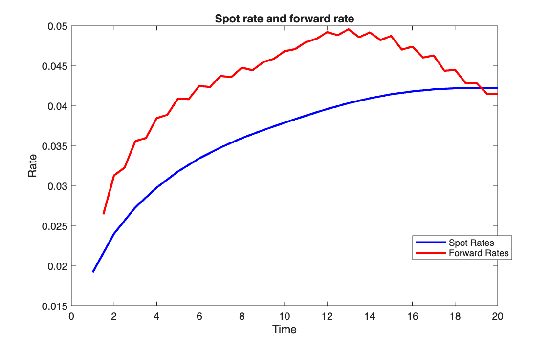
The swap rates go from 1.92% at 1 year to 4.09% at 20 years. Through the bootstrap, the spot curve goes from 1.92% to 4.22%, and the forward curve moves between 2.6% and 5.0%.
What the comparison actually shows
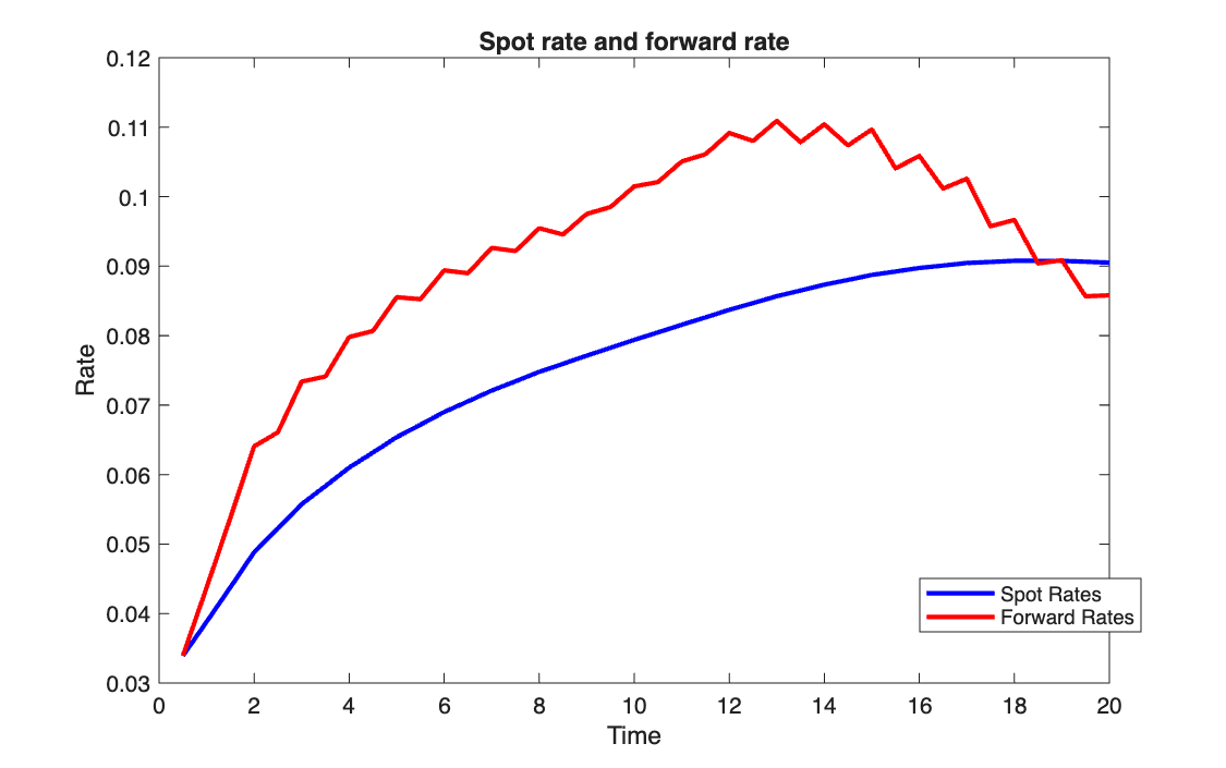
The second chart is off mainly for a different reason than the one stated in the code's
conclusion. The swap rates are interpolated to half-year steps, but F_es59 still
bootstraps them as annual swaps: each half-year is treated as a full year of coupon,
which roughly doubles the rates (9.05% at 20 years instead of 4.22%). Bootstrapping
the same interpolated rates with half-yearly coupons (\(z/2\)) gives 4.27% at 20 years,
almost the same as the correct procedure.
The zig-zag in the forward rates is present in both charts, with the same number of swings (23–24 changes of direction). It comes from the linear interpolation, whose slope changes at every original maturity, and forward rates, being marginal rates, amplify it.
Two smaller points: the first grid point (6 months) comes before the first swap maturity (1 year) and is not extrapolated in the correct procedure, so that curve starts at 1 year; and the choice between interpolating yields and swap rates matters much less than keeping the coupon frequency consistent.
Takeaways
- The order of operations is: bootstrap on the maturities that are actually quoted, then interpolate yields, then compute what you need on the finer grid.
- Every step must keep the same time convention: a formula written for annual coupons cannot be run on a half-yearly grid unchanged.
- Forward rates are the most sensitive output of a curve: any kink in the interpolation shows up there first.