Payoffs of option strategies¶

Course exercise 39 · Part I

Problem¶

Plot the payoff at maturity of five classic option strategies, built from European calls and puts: bull spread, bear spread, butterfly spread, straddle and strangle.

Method¶

At maturity, with underlying price \(S\) and strike \(K\):

\[ c(S) = \max(S - K,\, 0), \qquad p(S) = \max(K - S,\, 0) \]

Each strategy is a sum of these, long (+) or short (−):

Strategy	Construction	View
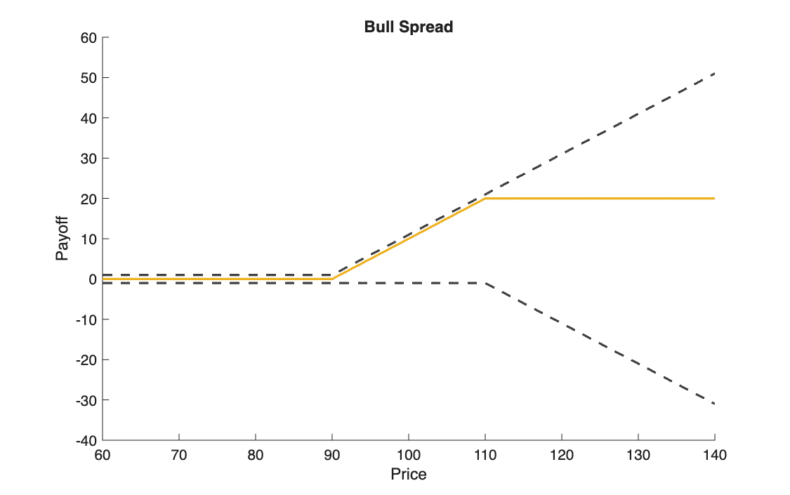
Bull spread	\(+c(K_1) - c(K_2)\)	moderate rise
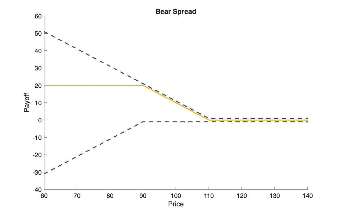
Bear spread	\(+p(K_2) - p(K_1)\)	moderate fall
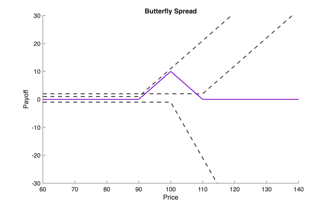
Butterfly	\(+c(K_1) - 2\,c(K_2) + c(K_3)\)	price stays near \(K_2\)
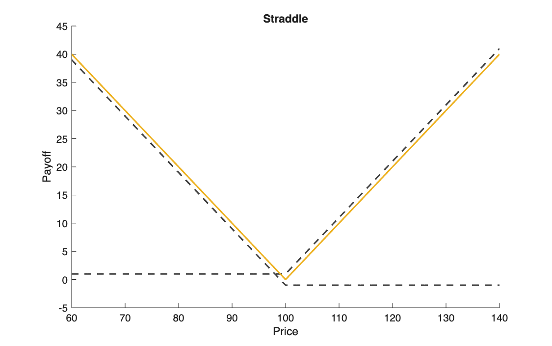
Straddle	\(+c(K) + p(K)\)	large move, either direction
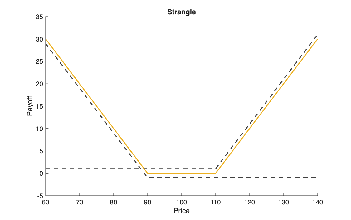
Strangle	\(+p(K_1) + c(K_2)\)	very large move, cheaper

Code¶

MATLABPython

S_exercise_39.m

clear all, clc

% Point 1
    % BULL SPREAD
    % A bet on a moderate rise in the price.
    % Buy a call with a low strike (K1) and finance it by selling a call
    % with a high strike (K2). Profit is capped, but so is the cost.

    S = 60:1:140;     % x axis: possible stock prices at maturity
    K_1 = 90;         % strike of the call you BUY
    K_2 = 110;        % strike of the call you SELL

    c_1 = max(S - K_1, 0); % payoff of the 90 call for each price in S
    c_2 = max(S - K_2, 0); % payoff of the 110 call for each price in S

    f_1 = c_1 - c_2;      % calculating Bull Spread strategy payoff

    % the payoffs of the strategy component have been shifted
    % to help the visualization of the strategy construction

    figure(1)
    hold on
    plot(S,c_1 +1,'--w',linewidth = 1.5)
    plot(S,-c_2 -1,'--w',linewidth = 1.5)
    plot(S,f_1,linewidth = 1.5)
    xlabel('Price')
    ylabel('Payoff')
    title('Bull Spread')
    hold off


% Point 2
    % BEAR SPREAD
    % A bet on a moderate fall in the price.
    % Buy a put with a high strike (K2) and sell a put with a low strike (K1).
    % The mirror image of the Bull Spread: maximum profit if the price falls.

    K_1 = 90;
    K_2 = 110;

    c_1 = max(K_1 - S, 0);
    c_2 = max(K_2 - S, 0);

    f_2 = c_2 - c_1;        % Bear Spread strategy payoff

    % the component payoffs are shifted to make the construction visible

    figure(2)
    hold on
    plot(S,-c_1 -1,'--w',linewidth = 1.5)
    plot(S,c_2 +1,'--w',linewidth = 1.5)
    plot(S,f_2,linewidth = 1.5)
    xlabel('Price')
    ylabel('Payoff')
    title('Bear Spread')
    hold off


% Point 3
    % BUTTERFLY SPREAD
    % A neutral strategy that bets on LOW VOLATILITY.
    % It pays off if the price at maturity stays close to the middle strike (K2).
    % The structure (1 long K1, 1 long K3, 2 short K2) gives up the profit if
    % the price moves too far from the centre, but also caps the loss.

    K_1 = 90;
    K_3 = 110;
    K_2 = (K_1 + K_3) / 2;

    c_1 = max(S - K_1, 0);
    c_2 = max(S - K_2, 0);
    c_3 = max(S - K_3, 0);

    f_3 = c_1 + c_3 - 2 * c_2;      % Butterfly Spread strategy payoff

    % the component payoffs are shifted to make the construction visible

    figure(3)
    hold on
    plot(S, c_1 + 1, '--w', 'LineWidth', 1.5)
    plot(S, -2 * c_2 - 1, '--w', 'LineWidth', 1.5)
    plot(S, c_3 + 2, '--w', 'LineWidth', 1.5)
    plot(S, f_3, 'LineWidth', 1.5)
    ylim([-30, 30])
    xlabel('Price')
    ylabel('Payoff')
    title('Butterfly Spread')
    hold off


% Point 4
    % STRADDLE (a bet on volatility)
    % Buy both a call and a put with the SAME strike (K).
    % It pays off if the price moves STRONGLY in either direction.
    % Expensive, because two premiums are paid.

    K = 100;

    c = max(S - K, 0);
    p = max(K - S, 0);

    f_4 = c + p;      % Straddle strategy payoff

    % the component payoffs are shifted to make the construction visible

    figure(4)
    hold on
    plot(S, c + 1, '--w', 'LineWidth', 1.5)
    plot(S, p - 1, '--w', 'LineWidth', 1.5)
    plot(S, f_4, 'LineWidth', 1.5)
    xlabel('Price')
    ylabel('Payoff')
    title('Straddle')
    hold off


% Point 5
    % STRANGLE (a cheaper bet on volatility)
    % Like the Straddle, but with different strikes (put at low K1, call at high K2).
    % Cheaper than the Straddle (lower premiums), but it needs a much larger
    % price move to become profitable.

    K_1 = 90;
    K_2 = 110;

    p = max(K_1 - S, 0);
    c = max(S - K_2, 0);

    f_5 = c + p;      % Strangle strategy payoff

    % the component payoffs are shifted to make the construction visible

    figure(5)
    hold on
    plot(S, c + 1, '--w', 'LineWidth', 1.5)
    plot(S, p - 1, '--w', 'LineWidth', 1.5)
    plot(S, f_5, 'LineWidth', 1.5)
    xlabel('Price')
    ylabel('Payoff')
    title('Strangle')
    hold off

S_exercise_39.py

import numpy as np
import matplotlib.pyplot as plt

S = np.arange(60, 141)                  # MATLAB: S = 60:1:140   (the end is excluded, hence 141)

# %% Point 1 - BULL SPREAD (buy call K1, sell call K2)

K_1 = 90
K_2 = 110

c_1 = np.maximum(S - K_1, 0)            # MATLAB: max(S - K_1, 0)   (np.maximum works element by element)
c_2 = np.maximum(S - K_2, 0)

f_1 = c_1 - c_2                         # Bull Spread payoff

# the component payoffs are shifted to make the construction visible
# ('--w', white, in the MATLAB version was meant for a dark background: black here)
plt.figure(1)
plt.plot(S, c_1 + 1, '--k', linewidth=1.5)
plt.plot(S, -c_2 - 1, '--k', linewidth=1.5)
plt.plot(S, f_1, linewidth=1.5)
plt.xlabel('Price')
plt.ylabel('Payoff')
plt.title('Bull Spread')

# %% Point 2 - BEAR SPREAD (buy put K2, sell put K1)

K_1 = 90
K_2 = 110

c_1 = np.maximum(K_1 - S, 0)
c_2 = np.maximum(K_2 - S, 0)

f_2 = c_2 - c_1                         # Bear Spread payoff

plt.figure(2)
plt.plot(S, -c_1 - 1, '--k', linewidth=1.5)
plt.plot(S, c_2 + 1, '--k', linewidth=1.5)
plt.plot(S, f_2, linewidth=1.5)
plt.xlabel('Price')
plt.ylabel('Payoff')
plt.title('Bear Spread')

# %% Point 3 - BUTTERFLY SPREAD (long K1, long K3, 2 short K2)

K_1 = 90
K_3 = 110
K_2 = (K_1 + K_3) / 2

c_1 = np.maximum(S - K_1, 0)
c_2 = np.maximum(S - K_2, 0)
c_3 = np.maximum(S - K_3, 0)

f_3 = c_1 + c_3 - 2 * c_2               # Butterfly Spread payoff

plt.figure(3)
plt.plot(S, c_1 + 1, '--k', linewidth=1.5)
plt.plot(S, -2 * c_2 - 1, '--k', linewidth=1.5)
plt.plot(S, c_3 + 2, '--k', linewidth=1.5)
plt.plot(S, f_3, linewidth=1.5)
plt.ylim([-30, 30])
plt.xlabel('Price')
plt.ylabel('Payoff')
plt.title('Butterfly Spread')

# %% Point 4 - STRADDLE (call + put, same strike)

K = 100

c = np.maximum(S - K, 0)
p = np.maximum(K - S, 0)

f_4 = c + p                             # Straddle payoff

plt.figure(4)
plt.plot(S, c + 1, '--k', linewidth=1.5)
plt.plot(S, p - 1, '--k', linewidth=1.5)
plt.plot(S, f_4, linewidth=1.5)
plt.xlabel('Price')
plt.ylabel('Payoff')
plt.title('Straddle')

# %% Point 5 - STRANGLE (put K1 + call K2)

K_1 = 90
K_2 = 110

p = np.maximum(K_1 - S, 0)
c = np.maximum(S - K_2, 0)

f_5 = c + p                             # Strangle payoff

plt.figure(5)
plt.plot(S, c + 1, '--k', linewidth=1.5)
plt.plot(S, p - 1, '--k', linewidth=1.5)
plt.plot(S, f_5, linewidth=1.5)
plt.xlabel('Price')
plt.ylabel('Payoff')
plt.title('Strangle')

plt.show()

Results¶

The solid line is the strategy; the dashed lines are its components, shifted up or down by one or two units so that they do not overlap.

Takeaways¶

These are payoffs, not profits: the premiums paid and received are not included.
The spreads cap both gain and loss at \(K_2 - K_1 = 20\); the butterfly peaks at \(K_2 - K_1 = 10\) exactly at \(S = K_2\).
Straddle and strangle are bets on volatility, not direction: the strangle needs a bigger move, because nothing pays between \(K_1\) and \(K_2\).