Mean-variance efficient frontier¶

Course exercise 131 · Part II

Problem¶

From five years of weekly prices of the EURO STOXX 50 constituents (47 stocks, 262 weekly returns), build the Markowitz efficient frontier with no short selling.

Method¶

With expected returns \(\mu\) and covariance matrix \(\Sigma\) estimated from the returns, each point of the frontier is the minimum-variance portfolio for a target return \(\eta\):

\[ \min_x\ x^\top \Sigma\, x \quad \text{s.t.} \quad \mu^\top x = \eta,\quad \mathbf{1}^\top x = 1,\quad x \ge 0 \]

The range of targets goes from the return of the global minimum-variance portfolio (solved with the budget constraint only) to the highest single-stock return, where the only feasible portfolio is that stock alone. quadprog minimises \(\tfrac12 x^\top H x\), so \(H = 2\Sigma\) makes its objective value exactly the portfolio variance.

Code¶

MATLABPython

S_exercise_131.m

clear all, clc

%% 1

A = readtable('weekly_EUROSTOXX50_price_time.txt');

%% 2

times = A{:, 1};
P = A{:, 2:end};

%% 3

RR = diff(P) ./ P(1:end-1, :);

%% 4

mu = mean(RR);
cov_ = cov(RR);
%
[n_valori, n_asset] = size(RR);
%

%% 5

% minimum risk portfolio

H = 2 * cov_;
Aeq = ones(1, n_asset);
beq = 1;
lb = zeros(n_asset, 1);

[x_min, var_min] = quadprog(H,[],[],[],Aeq,beq,lb,[])

eta_min = mu * x_min % return of the minimum risk portfolio

% maximum risk portfolio

eta_max = max(mu)

%% 6

eta = linspace(eta_min, eta_max, 100);

%% 7

options = optimset(MaxIter=1.e7, TolFun=1.e-10, TolX=1.e-10)

Aeq_ = [mu; ones(1, n_asset)]

for k = 1 : length(eta)
    beq_ = [eta(k) ; 1]
    [x_(:, k), var_(:, k)] = quadprog(H,[],[],[],Aeq_,beq_,lb,[],[],options)
end

%% 8

 save('MarkRiskyAsset.mat','var_', 'RR', 'eta')

%% 9

figure(1)
plot(var_, eta, lineWidth=2)
xlabel('Risk')
ylabel('Returns')
title('Efficient frontier')
print('Markowitz_EF.jpg','-djpeg')

S_exercise_131.py

import numpy as np
import matplotlib.pyplot as plt
from scipy.optimize import minimize     # scipy has no quadprog: minimize does the same job
from scipy.io import savemat

# %% 1
A = np.loadtxt('weekly_EUROSTOXX50_price_time.txt')   # MATLAB: readtable(...)   (a plain table of numbers)

# %% 2
times = A[:, 0]                         # MATLAB: A{:, 1}
P = A[:, 1:]                            # MATLAB: A{:, 2:end}

# %% 3
RR = np.diff(P, axis=0) / P[:-1, :]     # MATLAB: diff(P) ./ P(1:end-1, :)   (axis=0: along the rows)

# %% 4
mu = np.mean(RR, axis=0)                # one mean per stock (column)
cov_ = np.cov(RR, rowvar=False)         # MATLAB: cov(RR)

n_valori, n_asset = RR.shape

# %% 5 - minimum risk portfolio
H = 2 * cov_
obj = lambda x: 0.5 * x @ H @ x         # what quadprog minimises: here it equals the portfolio variance
lb = [(0, None)] * n_asset              # no short selling
budget = {'type': 'eq', 'fun': lambda x: np.sum(x) - 1}   # weights sum to 1
x0 = np.ones(n_asset) / n_asset         # starting point (quadprog does not need one, minimize does)

res = minimize(obj, x0, method='SLSQP', bounds=lb, constraints=[budget], options={'ftol': 1e-12, 'maxiter': 1000})
x_min = res.x
var_min = res.fun
print("var_min =", var_min)

eta_min = mu @ x_min                    # return of the minimum risk portfolio
print("eta_min =", eta_min)

# maximum risk portfolio
eta_max = np.max(mu)
print("eta_max =", eta_max)

# %% 6
eta = np.linspace(eta_min, eta_max, 100)

# %% 7
x_ = np.zeros((n_asset, len(eta)))
var_ = np.zeros(len(eta))

for k in range(len(eta)):
    target = {'type': 'eq', 'fun': lambda x: mu @ x - eta[k]}   # MATLAB: Aeq_ = [mu; ones], beq_ = [eta(k); 1]
    res = minimize(obj, x0, method='SLSQP', bounds=lb, constraints=[budget, target], options={'ftol': 1e-12, 'maxiter': 1000})
    x_[:, k] = res.x
    var_[k] = res.fun

# %% 8
savemat('MarkRiskyAsset.mat', {'var_': var_, 'RR': RR, 'eta': eta})   # MATLAB: save('MarkRiskyAsset.mat', ...)

# %% 9
plt.figure(1)
plt.plot(var_, eta, linewidth=2)
plt.xlabel('Risk')
plt.ylabel('Returns')
plt.title('Efficient frontier')
plt.savefig('Markowitz_EF.jpg')         # MATLAB: print('Markowitz_EF.jpg', '-djpeg')
plt.show()

Results¶

	Weekly return	Weekly variance	Weekly volatility
Minimum-variance portfolio	0.275%	0.000231	1.52%
Top of the frontier (single stock)	0.660%	0.000785	2.80%

The minimum-variance portfolio holds 18 of the 47 stocks.

Mean-variance efficient frontier

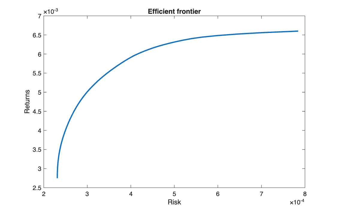
The horizontal axis is the portfolio variance, not the volatility.

Takeaways¶

The frontier is concave: the first units of extra return are cheap in risk, the last ones very expensive, because diversification is progressively given up.
Without short selling the optimal portfolios are sparse: most stocks get zero weight even at the minimum-variance point.
Everything rests on \(\mu\) and \(\Sigma\) estimated from 262 observations for 47 stocks; the frontier is only as reliable as those estimates.