Mean-MAD efficient frontier¶

Course exercise 135 · Part II

Problem¶

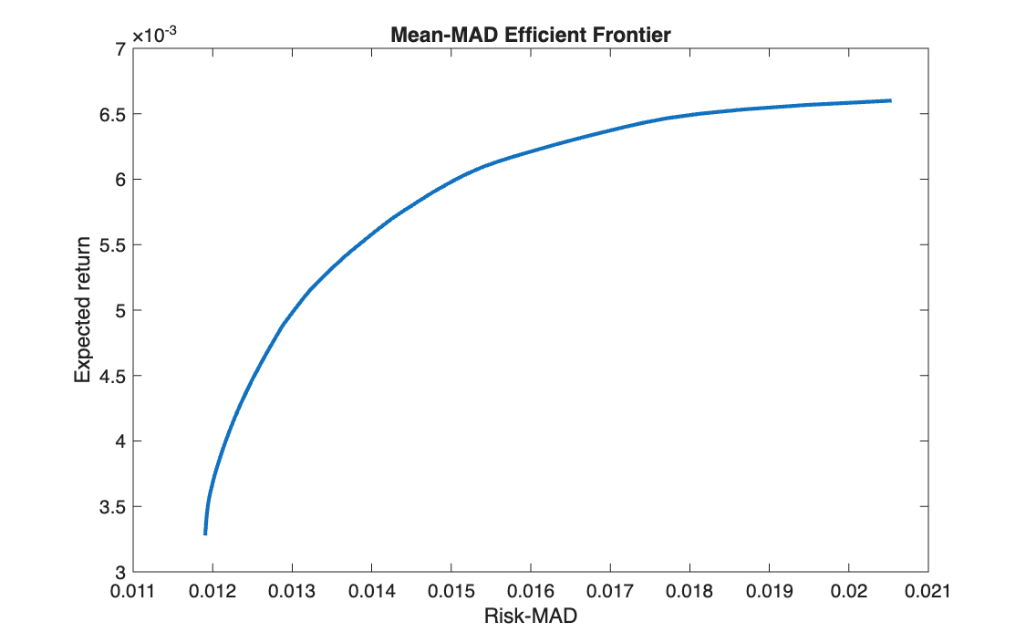
On the same EURO STOXX 50 data as the Markowitz frontier, replace variance with the mean absolute deviation (MAD) as the measure of risk, and build the corresponding efficient frontier.

Method¶

The MAD of a portfolio over \(T\) historical scenarios is \(\frac{1}{T}\sum_t \big| (r_t - \mu)^\top x \big|\). The absolute value is not linear, but it becomes linear with one auxiliary variable \(y_t \ge 0\) per scenario:

\[ \min_{x,\,y}\ \frac{1}{T}\sum_{t=1}^{T} y_t \quad \text{s.t.} \quad -y_t \le (r_t - \mu)^\top x \le y_t,\quad \mu^\top x = \eta,\quad \mathbf{1}^\top x = 1,\quad x \ge 0 \]

At the optimum each \(y_t\) equals the absolute deviation, so the whole problem is a linear program, solved with linprog for 100 target returns.

Code¶

MATLABPython

S_exercise_135.m

clear all, clc

%% 1

A = readtable("weekly_EUROSTOXX50_price_time.txt");
times = A{:, 1};
P = A{:, 2:end};

%% 2

RR = diff(P) ./ P(1:end-1, :);
[T, n] = size(RR);

%% 3

mu = mean(RR);

%% 4

dev = RR - repmat(mu, T, 1); % how far each return is from its mean

f  = [zeros(1, n), ones(1, T)/T];

A = [ dev,  -eye(T);
      -dev,  -eye(T)];
b  = zeros(2 * T, 1);

lb = zeros(n + T, 1);

% minimum risk (budget constraint only, no return constraint)
Aeq = [ones(1, n), zeros(1, T)];
beq = 1;

[port_min, mad_min] = linprog(f, A, b, Aeq, beq, lb, []);
x_min   = port_min(1:n);
eta_min = mu * x_min;
eta_max = max(mu);

%% 5

N   = 100;
eta = linspace(eta_min, eta_max, N);

%% 6

Risk_MAD = NaN(1, N);

Aeq_ = [mu,          zeros(1, T);
        ones(1, n),  zeros(1, T)];

for k = 1:N
    beq_ = [eta(k); 1];
    [port_k, mad_k] = linprog(f, A, b, Aeq_, beq_, lb, []);
    Risk_MAD(k) = mad_k;
end

%% 7

figure(1)
plot(Risk_MAD, eta, LineWidth=2)
xlabel('Risk-MAD')
ylabel('Expected return')
title('Mean-MAD Efficient Frontier')

S_exercise_135.py

import numpy as np
import matplotlib.pyplot as plt
from scipy.optimize import linprog

# %% 1
A = np.loadtxt('weekly_EUROSTOXX50_price_time.txt')
times = A[:, 0]
P = A[:, 1:]

# %% 2
RR = np.diff(P, axis=0) / P[:-1, :]
T, n = RR.shape

# %% 3
mu = np.mean(RR, axis=0)

# %% 4
dev = RR - np.tile(mu, (T, 1))          # how far each return is from its mean

f = np.concatenate([np.zeros(n), np.ones(T) / T])   # MATLAB: [zeros(1, n), ones(1, T)/T]

A = np.block([[ dev, -np.eye(T)],       # MATLAB: [ dev, -eye(T); -dev, -eye(T)]
              [-dev, -np.eye(T)]])
b = np.zeros(2 * T)

lb = [(0, None)] * (n + T)

# minimum risk (budget constraint only)
Aeq = np.concatenate([np.ones(n), np.zeros(T)]).reshape(1, -1)   # one row
beq = [1]

res = linprog(f, A_ub=A, b_ub=b, A_eq=Aeq, b_eq=beq, bounds=lb)
port_min = res.x
mad_min = res.fun
x_min = port_min[:n]                    # MATLAB: port_min(1:n)
eta_min = mu @ x_min
eta_max = np.max(mu)

# %% 5
N = 100
eta = np.linspace(eta_min, eta_max, N)

# %% 6
Risk_MAD = np.zeros(N)

Aeq_ = np.vstack([np.concatenate([mu, np.zeros(T)]),           # MATLAB: [mu, zeros(1, T);
                  np.concatenate([np.ones(n), np.zeros(T)])])  #          ones(1, n), zeros(1, T)]

for k in range(N):
    beq_ = [eta[k], 1]
    res = linprog(f, A_ub=A, b_ub=b, A_eq=Aeq_, b_eq=beq_, bounds=lb)
    Risk_MAD[k] = res.fun

print("mad_min =", mad_min, " eta_min =", eta_min, " MAD at the top =", Risk_MAD[-1])

# %% 7
plt.figure(1)
plt.plot(Risk_MAD, eta, linewidth=2)
plt.xlabel('Risk-MAD')
plt.ylabel('Expected return')
plt.title('Mean-MAD Efficient Frontier')
plt.show()

Results¶

The minimum-MAD portfolio has a weekly MAD of 1.19% and an expected return of 0.328%, holding 13 stocks. At the top of the frontier the MAD is 2.05%.

Mean-MAD efficient frontier

Takeaways¶

Replacing variance with MAD turns a quadratic program into a linear one, at the cost of \(T\) extra variables and \(2T\) constraints.
MAD does not need a covariance matrix: it works directly on the historical scenarios.
It penalises deviations linearly rather than quadratically, so it is less driven by a few extreme weeks than variance is.