Spot and forward rates from zero-coupon prices
Problem
Write a function that computes forward prices and forward rates from a set of zero-coupon prices (exercise 55). Apply it to five prices on a half-yearly schedule, compute the spot rates and plot the two curves (exercise 56).
Method
\[
i_{spot}(t_k) = v_k^{-1/t_k} - 1, \qquad
v_{fwd}(t_{k-1}, t_k) = \frac{v_k}{v_{k-1}}, \qquad
i_{fwd}(t_{k-1}, t_k) = v_{fwd}^{-1/(t_k - t_{k-1})} - 1
\]
The forward rate is the rate agreed today for the period between \(t_{k-1}\) and \(t_k\).
Code
clear all, clc

t = [0.5, 1, 1.5, 2, 2.5];           % arbitrary schedule
v = [0.98, 0.96, 0.94, 0.925, 0.92]; % ZCB prices

% Point 1
    spot_r = (1 ./ v).^(1 ./ t) - 1    % spot interest rates

% Point 2
    [fwd_p, fwd_r] = F_es55(v, t)

% Point 3
    plot(t, spot_r, 'r', LineWidth = 2);
    hold on;
    plot(t, fwd_r, '-w', LineWidth = 2);
    hold off;
    xlabel('Time');
    ylabel('Rate');
    title('Spot and forward rates', 'FontSize', 14);
    legend({'Spot Rates', 'Forward Rates'}, 'Location', 'southwest', 'FontSize', 16);
    % print('-dtiff', 'rates_graph');     % save the plot
function [fwd_p, fwd_r] = F_es55(v, t)

% inputs:   v := ZCB prices
%           t := the schedule

% outputs:  fwd_p := forward prices
%           fwd_r := forward interest rates

% v and t must have the same length!

n = length(v);

% Initialization
fwd_p = zeros(1, n); % preallocation
fwd_r = zeros(1, n); % preallocation

% Calculate the first element of fwd price and rate vectors
fwd_p(1) = v(1);
fwd_r(1) = (1 / fwd_p(1))^(1 / t(1)) - 1;

for k = 2:n
    fwd_p(k) = v(k) / v(k-1);
    fwd_r(k) = (1 / fwd_p(k))^(1 / (t(k) - t(k-1))) - 1;
end

end
import numpy as np
import matplotlib.pyplot as plt
from F_es55 import F_es55

t = np.array([0.5, 1, 1.5, 2, 2.5])            # arbitrary schedule
v = np.array([0.98, 0.96, 0.94, 0.925, 0.92])  # ZCB prices

# %% Point 1
spot_r = (1 / v) ** (1 / t) - 1                # spot interest rates
print("spot_r =", spot_r)

# %% Point 2
fwd_p, fwd_r = F_es55(v, t)
print("fwd_p =", fwd_p)
print("fwd_r =", fwd_r)

# %% Point 3
plt.plot(t, spot_r, 'r', linewidth=2)
plt.plot(t, fwd_r, 'k', linewidth=2)           # white ('-w') in the MATLAB version: black here
plt.xlabel('Time')
plt.ylabel('Rate')
plt.title('Spot and forward rates', fontsize=14)
plt.legend(['Spot Rates', 'Forward Rates'], loc='lower left', fontsize=16)
plt.show()
import numpy as np


def F_es55(v, t):
    # inputs:   v := ZCB prices
    #           t := the schedule (same length as v)
    # outputs:  fwd_p := forward prices
    #           fwd_r := forward interest rates

    n = len(v)

    fwd_p = np.zeros(n)                 # preallocation
    fwd_r = np.zeros(n)

    # first element: from today, the forward is the spot
    fwd_p[0] = v[0]                     # MATLAB: fwd_p(1) = v(1)   (the first element has index 0)
    fwd_r[0] = (1 / fwd_p[0]) ** (1 / t[0]) - 1

    for k in range(1, n):               # MATLAB: for k = 2:n
        fwd_p[k] = v[k] / v[k-1]
        fwd_r[k] = (1 / fwd_p[k]) ** (1 / (t[k] - t[k-1])) - 1

    return fwd_p, fwd_r
Results
| Maturity | ZCB price | Spot rate | Forward rate |
|---|---|---|---|
| 0.5 | 0.980 | 4.12% | 4.12% |
| 1.0 | 0.960 | 4.17% | 4.21% |
| 1.5 | 0.940 | 4.21% | 4.30% |
| 2.0 | 0.925 | 3.98% | 3.27% |
| 2.5 | 0.920 | 3.39% | 1.09% |
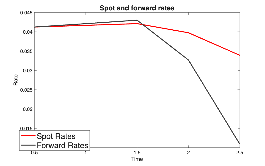
Takeaways
- The first forward rate equals the first spot rate: from today, there is no earlier period.
- When the spot curve rises the forward curve lies above it; when it falls, below. The forward is the marginal rate, the spot is the average.